Apr 24, 2020
Protocol for Geostatistical Determination of Radiation Dosimetry Maps of Population-Scale Exposures
- Eliseos Mucaki1,
- Peter Rogan1
- 1Western University


External link: https://doi.org/10.1371/journal.pone.0232008
Protocol Citation: Eliseos Mucaki, Peter Rogan 2020. Protocol for Geostatistical Determination of Radiation Dosimetry Maps of Population-Scale Exposures. protocols.io https://dx.doi.org/10.17504/protocols.io.ba4nigve
Manuscript citation:
A research article that describes this protocol is currently available as a pre-print:
Rogan PK, Mucaki EJ, Lu R, Shirley BC, Waller E, Knoll JHM. Meeting radiation dosimetry capacity requirements of population-scale exposures by geostatistical sampling. medRxiv 2020.04.08.20058446; doi: https://doi.org/10.1101/2020.04.08.20058446.
This manuscript has been accepted for publication in the journal PLOS ONE.
License: This is an open access protocol distributed under the terms of the Creative Commons Attribution License, which permits unrestricted use, distribution, and reproduction in any medium, provided the original author and source are credited
Protocol status: Working
We use this protocol and it's working
Created: January 08, 2020
Last Modified: April 24, 2020
Protocol Integer ID: 31598
Keywords: Humans, Radiation Dosage, Radiation Exposure, Software, Geostatistical Analysis, Simulation, Population Studies, Biodosimetry, Physical Dosimetry, Medical Emergency Management, radiation dosimetry maps of population, scale exposures accurate radiation dose estimate, radiation dosimetry map, spatial boundaries of graduated radiation exposure, accurate radiation dose estimate, scale radiation exposure, graduated radiation exposure, radiation exposure, established radiation dose, radiation dose, protocol for geostatistical determination, scale radiation event, physical radiation plume, geostatistical determination, geostatistical analysis of small population sample, nuclear detonation scenario, simulated exposure, throughput dosimetry analysis, nuclear spill incident, geostatistical analysis, critical locations for additional sampling, biodosimetry testing, scale exposure, empirical bayesian, small population sample, contours of successive plume
Abstract
Accurate radiation dose estimates are critical for determining eligibility for therapies by timely triaging of exposed individuals after large-scale radiation events. However, the universal assessment of a large population subjected to a nuclear spill incident or detonation is not feasible. Even with high-throughput dosimetry analysis, test volumes far exceed the capacities of first responders to measure radiation exposures directly, or to acquire and process samples for follow-on biodosimetry testing. We aimed to design a protocol which can significantly reduce data acquisition and processing requirements for timely treatment of eligible, affected individuals in population-scale radiation exposures.
Method in Brief: The spatial boundaries of graduated radiation exposures were determined by targeted, multistep geostatistical analysis of small population samples. Physical radiation plumes modelled nuclear detonation scenarios of simulated exposures at 22 US locations. Models assumed only location of the epicenter and historical, prevailing wind directions/speeds. Initially, locations proximate to these sites were randomly sampled (0.1% of population). Empirical Bayesian kriging established radiation dose contour levels circumscribing these sites. Densification of each plume identified critical locations for additional sampling. After repeated kriging and densification, overlapping grids between each pair of contours of successive plumes were compared based on their diagonal Bray-Curtis distances and root-mean-square deviations, which provided criteria (<10% difference) to discontinue sampling.
Guidelines
- If your intent is to eventually publish the images that you generate in ArcMap, we suggest using non-copyrighted background maps such as the Humanitarian Open Street Map. To use this map in ArcMap, open the ArcGIS Online dialog and search "humanitarian openstreetmap". Open the search result "OpenStreetMap Humanitarian" with the description "OpenStreetMap for Humanitarian Use".
Materials
MATERIALS
ArcMap 10 SoftwareESRICatalog #ESRI: Redlands, California
This protocol requires a license to the following software:
1) ArcMap or ArcGIS Pro (protocol tested on ArcMap v10.4).
2) ArcGIS Geostatistical Analysis toolbox
3) Access to ArcGIS Data Interoperability toolbox
4) Access to ArcGIS Spatial Analysis toolbox
Troubleshooting
Safety warnings
N/A
Before start
This protocol requires a license to the following software:
1) ArcMap or ArcGIS Pro (protocol tested on ArcMap v10.4).
2) ArcGIS Geostatistical Analysis toolbox
3) Access to ArcGIS Data Interoperability toolbox
4) Access to ArcGIS Spatial Analysis toolbox
Derivation and Processing of ground-truth HPAC radiation plumes
Nuclear detonation scenarios created by the Hazard Prediction and Capability software (HPAC; https://www.acq.osd.mil/ncbdp/nm/narp/Radiation_Data/Specialized_Radiological.htm) were derived for 22 North American cities and surrounding regions (simulations performed by the University of Ontario Institute of Technology (UOIT) Health Physics and Environmental Safety Research Group; plumes were simulated using HPAC v4.04 which models the dispersion of radiation (as well as chemical and biological releases) assuming only the location of the epicenter, historical prevailing wind direction and speeds, intensity and weather conditions). The files contain HPAC plume coordinate (WGS1984) and dose values (in cGy) for all scenarios discussed in the manuscript. Each scenario file has been made available in a Zenodo archive (https://doi.org/10.5281/zenodo.3572574):
Dataset
HPAC Plume Data (XML Format)
NAME
The plumes provided are in XML format, which is not compatible with ArcMap software (https://desktop.arcgis.com/en/arcmap/). To import this data into ArcMap, the XML files for the HPAC plume are first converted to a tab-delimited X,Y,Z format (Latitude, Longitude, and Dose) using a Perl script "XML-to-XY-Converter.Smooth-Circle-of-Zeros.All-Files.pl". This program also adds an unirradiated contour ("0 cGy") surrounding the HPAC plume, as the presence of unirradiated samples circumscribing the plume was found to be crucial for accurate dose estimation by kriging (see below). These 0 cGy locations serve as the geographic boundary for the kriging procedure.
This (and all other programs described in this protocol) can be found in the above mentioned Zenodo archive:
Dataset
Geostatistical Sampling Project: All Scripts
NAME
All HPAC scenarios that were processed by the aforementioned XML-to-XY-Converter program can be found in the Zenodo archive:
Dataset
HPAC Plume Data (Processed to Tab-Delimited Format)
NAME
Note: In this protocol, we provide images which illustrate the steps using the ArcMap software and custom software scripts to derive a radiation exposure map by geostatistical analysis of individual samples. These images are generated during the processing of a simulated nuclear incident scenario (single replicate) in the vicinity of Columbia, South Carolina , i.e. a worked example similar to those included in the accompanying manuscript.
Acquisition of United States (US) Census Data for Geostatistical Analysis
1. Download US state and sub-division boundary files (in KML [Keyhole Markup Language] format) from the US census bureau (https://www2.census.gov/geo/tiger/GENZ2016/shp/).
2. Determine the population of the regions surrounding the scenario of interest from: A) the US Census (“Incorporated Places and Minor Civil Divisions Datasets: Subcounty Resident Population Estimates: April 1, 2010 to July 1, 2017”), B) the American Fact Finder; and/or the Home Town Locator.
Processing and Import of US state and sub-division boundary files to ArcMap
Before importing the US state and sub-division boundary files to ArcMap, the KML files required editing. Exceptions handled US states with multiple sub-divisions that share the same name, so that ArcMap did not also select unintended sub-divisions found outside of the radiation plume. Sub-division names with spaces or dashes were also modified by concatenating them prior to ‘KMLtoLayer’ conversion to avoid their unintended truncation.
1. Correct KML files by using the script "KML-Name-Correcting-Program.pl" (available through Zenodo; https://doi.org/10.5281/zenodo.3572574). To run:
- Place program in folder with all KML files you wish to modify
- To Run: "perl KML-Name-Correcting-Program.pl"
2. Import the modified KML boundary files to ArcMap using the software's ‘KMLtoLayer’ tool (additional parameters are not required for this step). When this process finishes, the KML boundary file will be displayed on the map.
South Carolina boundary files displayed on the map using ArcMap v10.4.
3. Use ArcMap's "Split" command to allow ArcMap to be able to identify each sub-division within the boundary file, and allows the user to display specific subdivisions within the KML boundary file.
- "Input Features": Select the KML file of interest -> "Polygon"
- "Split Features": Repeat "Input Features" step (splitting the file on itself)
- "Split Field": Select "Name"
- "Target Workspace": Create a new Geodatabase (name it "StateName_Split"), highlight the Geodatabase and click "Add".
- "XY Tolerance": Leave blank
ArcMap 10.4 Dialog Box for the "Split" Command. 'Input Features' and 'Split Features' are assigned the KML boundary files imported by "KMLtoLayer" in section 2.1 step 2. "Split" will not work if you attempt to perform the split on KML files that are not imported first. Note that "cb_2016_45_cousub_500k" is the name of the KML boundary file which defines the borders and subdivisions of South Carolina.
Click OK. This process may take several minutes. When complete, click "Add Data" and open the newly created Geodatabase. This database will contain a file for each sub-division, which can be used for downstream steps.
South Carolina Geodatabase contains polygons for each sub-division of the state, which can now be selected individually after splitting.
Simulated analyses of population-scale, nuclear radiation scenarios
Creating a set of random locations, i.e. points, to simulate random sampling of 0.1% of the population in each geographic subdivision
- Upload the HPAC-generated radiation plume files for the scenario of interest on ArcMap (see Section 4 on how to add data to ArcMap) and visually determine which sub-divisions it overlaps.
- Use Census data to determine the population of each of these sub-divisions.
- Random sampling locations are created for each sub-division using the ArcMap tool, ‘CreateRandomPoints_management’. We created a Python script to perform this task manually. This python script has to be edited for each scenario, as users must manually select the subdivision and assign the number of random points for that sub-division (in our study, that number was 0.1% of the population of that sub-division; if sub-division is made up of multiple unconnected segments, the population was divided evenly between each part) in the Python code:
import arcpy
import sys
# where any output will be written
arcpy.env.workspace = "C:/PATH/TO/OUTPUT/WORKSPACE/"
# create 10 sets of random points
for x in range(0, 10):
# path to split KML Geodatabase from Section 2.1
outlocation = "C:/PATH/TO/KMLSplit/StateName_Split.gdb"
# repeat the following 2 lines for each subdivision of interest
featureclass = "C:/PATH/TO/KMLSplit/StateName_Split.gdb/Subdivision1Name"
arcpy.CreateRandomPoints_management(outlocation, "Subdivision1NameRandPts", featureclass, "", 465, "", "POINT") # where 465 is the number of random points to draw in this subdivision
# repeat above two lines for each subdivision of interest
# merge the random points as one file
merge_name = "MergedPoints%d" % x
arcpy.Merge_management(["Subdivision1Name", "Subdivision2Name", ...], merge_name)
# add XY coordinates to the created random points
arcpy.AddXY_management(merge_name)
4. Run the Python script through ArcMap (Geoprocessing -> Python)
- Type: execfile(r'C:/PATH/TO/SCRIPT/Random-Point-Generator-Program')
How to Execute Python scripts within ArcMap 10.4.
Program run time depends on the number of cycles assigned (each cycle is a completely different set of samples, used as separate "replicates" in our study), and the number of sub-divisions that the HPAC plume overlaps, but can take over an hour. ArcMap crashing during this process was a reoccurring problem. To alleviate this, we performed this step in 10-25 cycle batches. To perform a new set of cycles, save the completed batch of random sample locations, adjust the for loop in the code to include additional cycles (i.e. if for loop was set to "0, 25", we adjust the values to "26, 50"), and rerun the program in the Python window in ArcMap. Therefore, if the program crashes at this step, the initial batch or random s is still saved. If ArcMap does crash, open this latest save and re-run the script.
The program described above creates the random sample locations in ArcMap. Next, we extract these random sample locations and convert them into a text file format for downstream processing steps. To do so, we run the export Python script described below. This script was originally a part of the previously described Python script, but as ArcMap would often crash during this final step of the process, we decided to perform this task with a separate program explicitly written for this purpose. The following script is also provided in the Zenodo archive, under the name "Random-Point-Exporting-Script.py":
import arcpy
import sys
arcpy.env.workspace = "C:/Users/ROGANLAB/Desktop/HPAC-Data/Jacksonville_FL-DirectionChange"
# set for loop to the total number of cycles generated in the previous program
for x in range(0, 25):
merge_name = "MergedPoints%d" % x
output_file = "StateName_March_%d.txt" % x
arcpy.ExportXYv_stats(merge_name,"FID", "COMMA",output_file,"ADD_FIELD_NAMES")
Next, the random selected sample locations exported in Section 3 (or the densification-directed sampling locations selected by densification; see Section 5) are assigned radiation dose values corresponding to the adjacent outer HPAC contour. This is done by the script "XML-to-XY-Conversion.REM-Assigner.Multiple-Files.pl", which compares the location of a sample to its location relative to the HPAC plume (the processed HPAC plume data file from Section 1). The values assigned to these sample locations are meant to simulate the values obtained by dosimetry methods. This program, like all other scripts described in this protocol, is available in the Zenodo archive.
Note that the program must be edited to direct the program towards the following:
- "$filename" should be assigned the HPAC Plume the random locations are being assigned to (full path to file)
- "$randompointspath" should be assigned the path to the folder which contains each of the exported random point files
- To Run: "perl XML-to-XY-Conversion.REM-Assigner.Multiple-Files.pl"
The program creates text files (one for each input file) with a new column which assigns the random sample locations a radiation value (in cGy) based on its location relative to the HPAC plume it is being compared to. If the sample does not overlap the HPAC plume, it will be assigned a value of 0 cGy.
Empirical Bayesian kriging
The following section describes how to generate a plume in ArcMap using Empirical Bayesian kriging.
- Import the HPAC plume and/or the random point data (from Section 3.1) to ArcMap using the "Add Data" function
- Right-Click the imported data in the "Table of Contents" window, and select "Display XY Data..."
In the "Display XY Data" dialog box, assign the X Field "Longitude", the Y Field "Latitude" and the Z Field "Data". Then under "Description", click Edit. This will open the Spatial Reference Properties dialog box. Select: "Geographic Coordinate System" -> "World" -> "WGS 1984". Click OK. Then click OK in the original dialog box.
'Display XY Data' Dialog Box
- The imported data should now appear on the map, and a new "event" for this data should appear in the "Table of Contents". Right-click this event, and select "Zoom To Layer" to quickly orient the map to location of the imported data.
Open the Geostatistical Wizard (under the Geostatistical Analysis toolbar; if this does not appear, make sure the extension is activated under Customize -> Extensions). This will open a dialog box. On the right, select Geostatistical Methods -> Empirical Bayesian Kriging. Under "Input Data", select the event created in step 3 (the "Display XY Data" step) as your Source Dataset, and "Data" (or field 3 if your data doesn't have headers) as the Data Field. Click Next. We used default values for our analysis. Click Next again and then click Finish. A "Method Report" should appear on screen, and the Empirical Bayesian kriging-based plume should appear on the map.
Progression of Geostatistical Wizard when performing Empirical Bayesian kriging (from left to right).
- On the Table Of Contents, double-click the newly derived intermediate plume. Give the plume a specific name. Then under "Symbology", click "Classify". Under "Method", select Equal Intervals, and under classes, reduce to 7. This will change the plume to have a color assigned to 0-100 cGy, 100-200 cGy, 200-300 cGy, ... 600-700 cGy. This keeps plumes consistent, and allows for easier identification of the plume's 2 Gy threshold. We recommend assigning the 0-100 cGy symbol of the plume to "No Color", as this symbol essentially draws on the map where the plume is not located.
Dialog box for editing the symbols which represent each radiation level of the kriging layer. The "Classification" dialog box (right) is opened from the "Classify..." icon in the "Layer Properties" dialog box (red arrow; left). These symbols (and the ranges they signify) can be quite different when performing kriging on different data sets, so normalizing these ranges are important for maintaining consistency when comparing plumes.
Plume for the Columbia, South Carolina scenario, derived only from Random Points based on 0.1% of the population. The plume is poor due to a lack of samples, which is often the case in regions of low population density. To improve the plume, we progress to Section 5 where we determine new sampling locations using densification.
Determining New Sampling Locations using Densification
The “Densify Sampling Network” tool of the Geostatistical toolbox determine the lower confidence regions in the kriging-derived map, i.e. regions with highest variance specifying radiation dose. We applied this tool to limit results to regions that would most likely exceed a pre-defined radiation level threshold (2Gy). In practice, the locations selected by densification would be used to direct first responders to new locations for subsequent rounds of data acquisition in order to improve the accuracy of the kriging-derived map.
- In the Geostatistical Toolbox, select "Densify Sampling Network". This will open a dialog box.
- Under "Input Geostatistical Layer", select the plume generated in Section 4.
- Under "Number of output points", we chose 200. This will generate 200 new sampling locations.
- Under "Selection Criteria", select the QUARTILE_THRESHOLD_UPPER option
- Under "Threshold Value", select 200 (will place points near regions expected to have a 200 cGy [2Gy] level of radiation, based on the current iteration of the plume)
(Optional) Adding an inhibition distance of 1 meter eliminates the issue where densification selects the same location multiple times.
'Densify Sampling Network' dialog box on ArcMap 10.4.
- When densification is complete, we add coordinates to the densification-directed sampling locations using the ArcMap function "Add XY Coordinates" (under the Data Management toolbox) as they are not automatically assigned. Simply select the output from the densification step as the input for this step and click OK. This step takes 10-20 seconds.
Export the data. Right-click the densification result in the Table of Contents and select "Open Attributes Table". Click the top left drop-down menu and select Export. Click the folder icon under 'Output Table' and change "Save as Type" to Text File, and give the file a name.
Exporting densify-directed sampling locations as a text file from the Attributes Table in ArcMap 10.4. The 'Export Data' dialog box (top right) is opened from the drop-down menu from the Attributes Table (left). The 'Saving Data' dialog box (bottom right) is opened when clicking the folder icon within the 'Export Data' dialog box.
- Repeat Section 3.1 for the exported file to assign the densification-directed sampling locations radiation values based on their location relative to the HPAC plume.
- Combine the new sampling locations with the initial set of sampling locations (simply combine the two files).
- Repeat Section 4 to generate a new plume, based on both the initial sampling data points and the new densification-directed sampling locations.
Densification is a compute intensive step, requiring approximately 1 hour on a desktop with an Intel i7-4770 processor [3.4Ghz] and 16GB of RAM. Note that reducing the number of requested sampling locations decreases overall processing time.
Intermediate Stage Plume for the Columbia, South Carolina scenario, initially derived from Random Sample locations, and followed by 1 iteration of kriging and densification. The kriging layer now better resembles a plume (though it is not yet contiguous), but can be further improved with additional kriging and densification iterations (see Section 6).
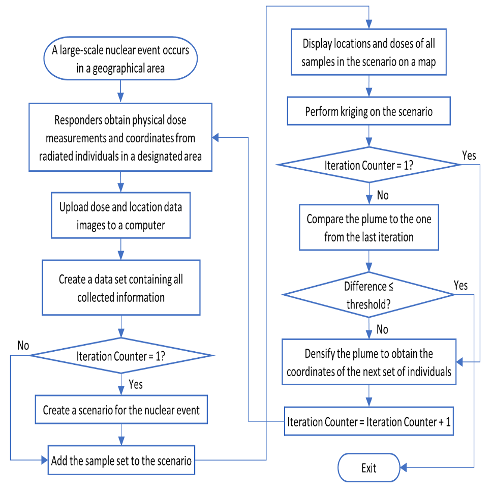
Radiation Plume Reconstruction with Iterative Kriging and Densification
The steps described in Section 3 are meant to simulate an initial batch of samples after a nuclear event, while the steps described in Section 5 are meant to simulate additional sampling data from locations assigned by the ArcMap software. While the samples from Section 3 create an initial plume, the combination of the data points from Section 3 and Section 5 create a second, much more accurate plume (see the final figure in Section 5). The plume is improved further when Sections 4 and 5 are repeated. These is referred to as an "iteration" of our protocol.
The iterative workflow for handling a population-scale radiation event. First responders collect physical dose measurements and location coordinates of the tested individuals. Measurements are then collected and mapped. A dose plume is generated, and densification is used to determine optimal locations for follow-up sampling. These steps are repeated until output dosimetry plume converges, and can be used to identify areas of ≥2Gy doses. The individuals residing in this part are eligible to be treated by cytokine therapies.
The first derived plume is based only on the initial random sampling locations: Sections 3 -> 3.1 -> 4. The first iteration is a combination of the initial sampling and additional sampling locations based on the first densification step: Sections: 3 -> 3.1 -> 4 (first plume generated) -> 5 -> 3.1 -> 4 (second plume generated).
Each additional iteration consists of repeating Sections 5 -> 3.1 -> 4 (Perform densification -> Determine new location's radiation value -> Combine new points with all previous samples -> Perform Kriging on all available sample data). This iterative process is continued until the latest plume is not significantly different from the plume generated in the previous iteration. To determine if the iterative process is no longer significantly changing the plume, see the next section (6.1).
Intermediate Plume for the Columbia, South Carolina scenario, derived from Random Points, followed by 5 iterations of kriging and densification.
How to Compare Two Plumes to Each Other
Plume comparisons are performed for the following two tasks:
- Determine if additional kriging and densification does not improve geographic coverage relative to the previous plume iteration
- Determine the accuracy of the plume relative to the HPAC plume
The actual steps to perform these two tasks are similar to one another: 1) Use kriging to generate a layer (which represents a radiation plume) to be compared [previous iteration to current iteration; or current iteration to HPAC plume]; 2) Convert those plumes into polygons; 3) Create a Union of the two polygons; 4) Use "Shape_Area" to compute the amount of overlap between the different levels of radiation between the two plumes.
- Use kriging to generate each plume, as described in Section 4. It is crucial that the "Class" [radiation levels] are the same between the two plumes.
- In ArcMap, perform "GA Contour to Layer" (Geostatistical Analyst toolbox) twice for each kriging layer to be compared. In the opened dialog box, select the kriging layer for the "Input Geostatistical Layer", with "Contour Type" as "SAME_AS_LAYER". Click Classification to expand the window. Under Classification Type, select Equal Interval. Click OK. Repeat for the second kriging layer.
- In ArcMap, perform "Feature To Polygon" (Data Management toolbox) twice for each contour generated in the previous step. Simply select the contour in the previous section and click OK. Repeat for the second kriging layer.
- (optional) Unfortunately, when creating the polygon, the radiation level assigned to each contour is lost. To add this back, right-click the polygon file in the Table of Contents and click Open Attributes Table. Add a new column. For each line, type in the radiation value (determine this by clicking the line and observing the highlighted region of the plume on the map). Repeat for the second polygon.
Create a Union between the two polygons: Geoprocessing -> Union. In the dialog box, select each polygon to be combined. The order in which the polygon is selected affects the order they will appear in the Attributes Table, so be mindful (e.g. for consistency, I always pick the current iteration of the plume second).
'Union' dialog box on ArcMap 10.4. The order Features are selected influence the order in which the overlapping appear in the Attributes table (attributes first selection will be on the left).
- Right-click the Union in the Table of Contents, and click Open Attributes Table. Each line represents a region where the two plumes overlapped. Export this table as described in Section 5. Open the file in Excel.
Union of the HPAC plume and the intermediate plume for the Columbia South Carolina scenario.
The protocol diverges in the analysis of the Union between the two plumes. When comparing two iterations of the derived plume (in Excel):
- Order the columns in terms of increasing radiation values for one of the plumes.
- For each radiation level for one plume, determine whether the intersecting region of the second plume has the same radiation value. Sum the Shape_Area column for the intersecting segments of the plume where the radiation level matches, as well as the intersecting segments that do not match. Determine the percentage of the area of the two intersecting plumes that are in agreement (have the same radiation level) by dividing the Shape_Area of matching intersecting segments by the sum of the matching and non-matching segments (which should equal the total area of that radiation level for the first plume).
- If the area of the radiation level of a contour of one plume exceeds 90% of the area of the other plume over all radiation levels, then the iterative process is discontinued (the 90% threshold can be changed by the user).
Comparing the current iteration of the radiation plume with the HPAC plume is similar to comparing plumes from consecutive iterations, but we instead group the regions of each plume that are above and below 2Gy (or 200 cGy), which was a threshold selected based on US government recommendations for eligibility of clinical treatment of acute radiation syndrome by cytokine therapies.
- Determine the regions of overlap between the HPAC and the intermediate plume that both represent a radiation value ≥ 2Gy, and sum the Shape_Area of each overlap.
- Determine the regions of overlap where the HPAC plume represents a radiation level ≥ 2Gy but the intermediate plume represents a radiation level < 2 Gy, and sum the Shape_Area of each overlap.
- Compute the accuracy of the intermediate plume by dividing the total Shape_Area of the overlapping ≥ 2Gy regions (Step 1) with the total Shape_Area of the HPAC plume's regions ≥ 2Gy (Step 1 + Step 2).
Comparison of the HPAC plume and the intermediate plume derived after 5 iterations of the protocol. Yellow highlights regions of the HPAC plume ≥ 2Gy which overlaps regions of the intermediate plume ≥ 2Gy, while orange highlights regions where the HPAC plume is ≥ 2Gy but the intermediate plume is < 2Gy. The accuracy is computed by taking the sum of the Shape_Area of the overlapping regions ≥ 2Gy and dividing it by the Shape_Area of the regions of the HPAC plume ≥ 2Gy only (the sum of the yellow and orange highlighted regions). In this Columbia South Carolina scenario replicate, we obtained an ≥ 2Gy accuracy of 68.4%.