Jul 03, 2025
Predictive modelling of Dirofilaria repens distribution in Russia
- Yury Prilepsky1,2,
- Sergey Konyaev1,3
- 1Institute of Systematics and Ecology of Animals of the Siberian Branch of the RAS, Novosibirsk, Russian Federation;
- 2e-mail: [email protected];
- 3e-mail: [email protected]
- Yury Prilepsky: conception, design; acquisition of data; creation of R script;
- Sergey Konyaev: validation of the protocol, acquisition of data;


Protocol Citation: Yury Prilepsky, Sergey Konyaev 2025. Predictive modelling of Dirofilaria repens distribution in Russia. protocols.io https://dx.doi.org/10.17504/protocols.io.kqdg3wznpv25/v1
License: This is an open access protocol distributed under the terms of the Creative Commons Attribution License, which permits unrestricted use, distribution, and reproduction in any medium, provided the original author and source are credited
Protocol status: Working
We use this protocol and it's working
Created: June 01, 2025
Last Modified: July 03, 2025
Protocol Integer ID: 219292
Keywords: Russia, ENM, Distribution, Machine learning, SDM, R, Dirofilaria, Dirofilaria repens, Parasite, predictive modelling of dirofilaria repens distribution, comprehensive ecological niche modeling approach, dirofilaria repens distribution, dirofilaria, repens across russia, multiple machine learning, using multiple machine learning, predictive modelling
Funders Acknowledgements:
Federal Basic Scientific Research Program
Grant ID: FWGS-2021-0001
Abstract
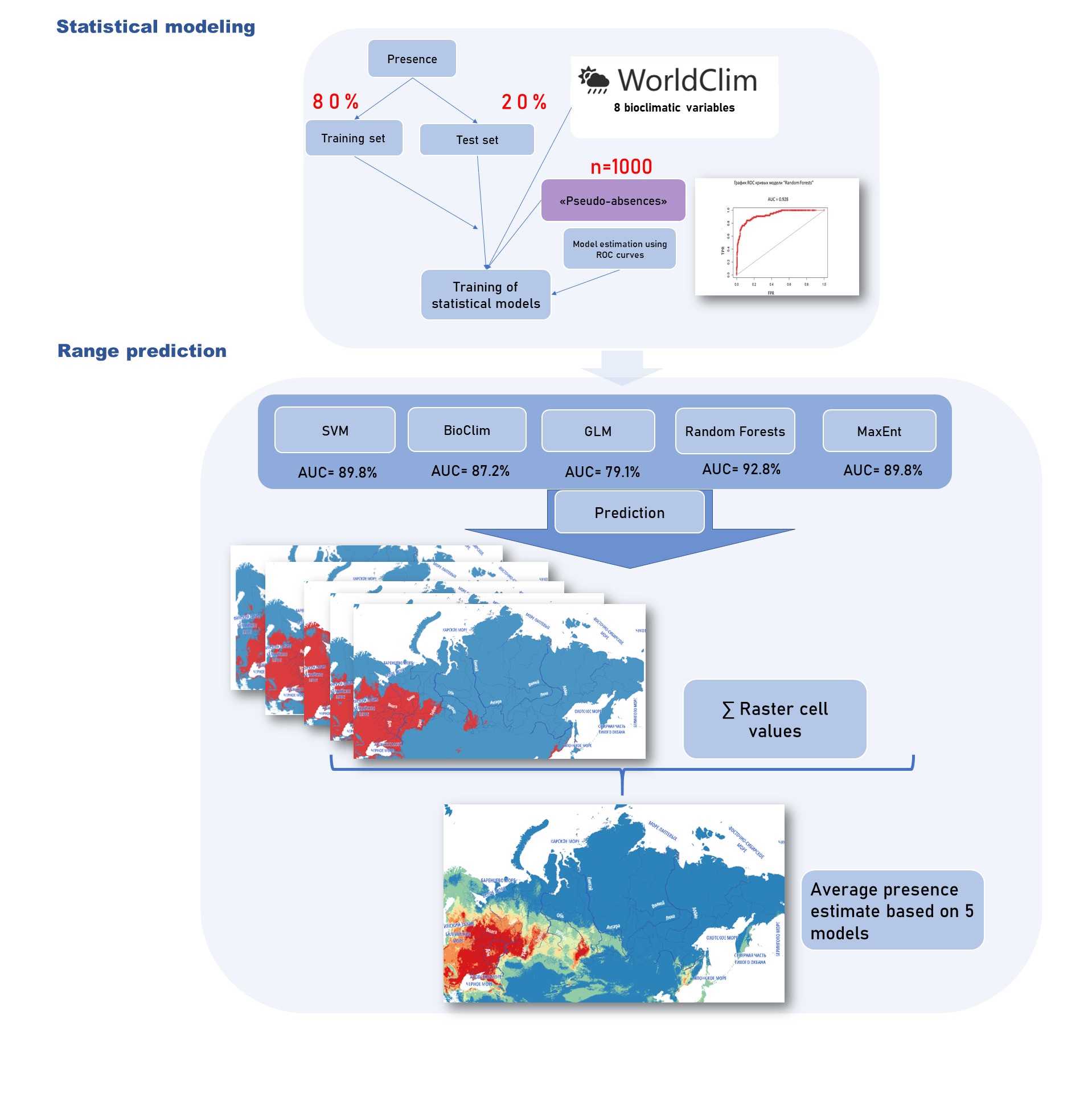
This protocol details a comprehensive ecological niche modeling approach to predict the distribution of Dirofilaria repens across Russia using multiple machine learning algorithms.
Image Attribution
The study design outlining how species occurrence data is utilized to forecast species distribution using statistical models driven by climatic data.
Guidelines
Extensive research conducted across the Russian Federation reports the presence of Dirofilaria repens (Sergiev et al. 2012), primarily in the southwestern part of the country, where the human population is concentrated. Ecological niche modeling is used to predict the parasite's occurrence in various regions with diverse orography and climatology at local, continental, and global levels. Considering these factors, the aim of this study was to develop ecological models that would most accurately predict the range of Dirofilaria repens. A broad set of variables related to parasite transmission was used. Climatic parameters (Bio_1-Bio_17) were obtained from the World Clim website (Fick and Hijmans 2017).
Various algorithms were employed in species distribution modeling. They can be classified as "profile", "regression," and "machine learning" methods. Profile methods consider only "presence" data. Regression and machine learning methods use both presence and absence or background data. Different algorithms have varying predictive capabilities and rely on different statistical principles, so their combined use can help achieve the most objective understanding of the current distribution of Dirofilaria repens.
Before start
Before proceeding with the analysis, it is necessary to download raster climate data from the WorldClim project website at the required spatial resolution.
To streamline the workflow, we recommend:
1. Creating a dedicated working directory for each project.
2. Setting this directory as the working directory in R (e.g., using setwd() function or RStudio projects).
This approach ensures organized file management and reproducibility
Data Preparation
To build the models, we used predictors representing climatic data in raster formats, as well as data on the presence of Dirofilaria repens in dog blood from various cities in Russia.
options(java.parameters = c("-XX:+UseConcMarkSweepGC", "-Xmx16g"))
gc()
library(dismo)
library(maptools)
library(kernlab)
library(raster)
library(car)
library(randomForest)
library(ggplot2)
library(rasterVis)
library(terra)
library(tidyverse)
library(geodata)
library(tidyterra)
setwd ("YOUR_PROJECT_DIRECTORY")
ext <- extent(20, 180, 35, 80)
predictors <- stack(list.files("/predictors", pattern='tif$', full.names=TRUE), quick=T)
predictors_maxent <- stack(list.files("/Maxent_predictors", pattern='tif$', full.names=TRUE), quick=T)
file <- file.path(getwd(), "PRESENCE_POINTS.csv")
dirofilaria <- read.table(file, header=TRUE, sep=',')
dirofilaria <- dirofilaria[,-3]
colnames(dirofilaria) = c('lon', 'lat')
To train the models, it is necessary to extract data on climatic parameters at the sample points.
set.seed(0)
presvals <- raster::extract(predictors, dirofilaria)
backgr <- dismo::randomPoints(predictors, 1000, ext = ext, p=dirofilaria, excludep = T, extf = 0.95)
absvals <- raster::extract(predictors, backgr)
pb <- c(rep(1, nrow(presvals)), rep(0, nrow(absvals)))
sdmdata <- data.frame(cbind(pb, rbind(presvals, absvals)))
pred_nf <- predictors
predictors_maxent <- predictors
Splitting presence points into training and test sets (80% and 20%, respectively)
set.seed(0)
group <- kfold(dirofilaria, 5)
pres_train <- dirofilaria[group != 1, ]
pres_test <- dirofilaria[group == 1, ]
Generating background points and splitting them into training and test sets (80% and 20%, respectively)
set.seed(0)
backg <- randomPoints(pred_nf, n=1000, ext=ext)
colnames(backg) = c('lon', 'lat')
group <- kfold(backg, 5)
backg_train <- backg[group != 1, ]
backg_test <- backg[group == 1, ]
r <- raster(pred_nf, 1)
| lon | lat | |
| 39.42597 | 47.11392 | |
| 39.86136 | 47.26870 | |
| 38.68672 | 50.62994 | |
| 37.31689 | 44.89427 | |
| 43.82109 | 55.39879 | |
| 41.12941 | 44.99936 |
Presence points of the species
The entire dataset was divided into training and test sets, and a background layer required for some algorithms was generated.
plot(!is.na(r), col=c('white', 'lightgrey'),ext=ext+5, legend=FALSE)
points(backg_train, pch='-', cex=0.5, col='yellow')
points(backg_test, pch='-', cex=0.5, col='black')
points(pres_train, pch= '+', cex=0.5, col='green')
Map with green dots indicating Dirofilaria repens presence and black/yellow dots indicating pseudo-absence test/train points needed for model fitting
Bioclim
The BIOCLIM algorithm is widely used for species distribution modeling. BIOCLIM is a classic "climate envelope" model (Busby 1991; Booth et al. 2014). Although it is generally not as good as some other modeling methods (Elith et al. 2006, 2011), especially in the context of climate change (Hijmans and Graham 2006), it is still used and can be useful for interpreting results from other studies. The BIOCLIM algorithm computes location similarity by comparing environmental variable values at any location to the percentile distribution of values at known occurrence locations ("training sites"). The closer to the 50th percentile (median), the more suitable the location. The tails of the distribution are not distinguished, meaning the 10th percentile is treated as equivalent to the 90th percentile. In the "dismo" implementation, values in the upper tail are transformed to the lower tail, and the minimum percentile score across all environmental variables is used. This value is subtracted from 1 and then multiplied by two, so the results range from 0 to 1. The reason for scaling this way is to make the results more similar to those of other distribution modeling methods, making them easier to interpret. A value of 1 will rarely be observed, as it would require a location with the median value of the training data for all considered variables. A value of 0 is very common, as it is assigned to all cells with an environmental variable value outside the percentile distribution (training data range) for at least one variable.
##Bioclim
bc <- bioclim(pred_nf, pres_train)
e_Bioclim <- evaluate(pres_test, backg_test, bc, pred_nf)
tr_biclim <- threshold(e_Bioclim, 'spec_sens')
pb <- predict(pred_nf, bc, ext=ext, progress='')
spplot(pb, main='Bioclim, raw values')
spplot(pb > tr_biclim, ext=extent(pb), main='presence/absence')
pb_bio <- pb > tr_biclim
The predictive capability of the model can be assessed using an ROC plot:
plot(e_Bioclim, "ROC")
Generalized Linear Model
The Generalized Linear Model (GLM) is an extension of ordinary least squares regression. The GLM function can be specified in various ways (Guisan, Edwards, and Hastie 2002), but in our case, the most accurate predictions are provided by a binomial logistic regression model.
To perform this, we refined our dataset and prepared it in a format suitable for the model-building function. The data structure can be seen in the table.
train <- rbind(pres_train, backg_train)
pb_train <- c(rep(1, nrow(pres_train)), rep(0, nrow(backg_train)))
envtrain <- raster::extract(predictors, train)
envtrain <- data.frame( cbind(pa=pb_train, envtrain) )
## Remove Na row's
envtrain <- envtrain[complete.cases(envtrain),]
testpres <- data.frame( raster::extract(predictors, pres_test))
testbackg <- data.frame( raster::extract(predictors, backg_test) )
testpres <- testpres[complete.cases(testpres),]
testbackg <- testbackg[complete.cases(testbackg),]
head(envtrain)
| pa<dbl> | bio_1<dbl> | bio_12<dbl> | bio_16<dbl> | bio_17<dbl> | bio_5<dbl> | bio_6<dbl> | bio_7<dbl> | bio_8<dbl> | |
| 1 | 9.908958 | 571 | 172 | 117 | 28.15700 | -6.563000 | 34.72000 | 20.21350 | |
| 1 | 12.302315 | 558 | 189 | 117 | 27.75556 | -1.288889 | 29.04445 | 4.72500 | |
| 1 | 3.454500 | 500 | 188 | 72 | 23.80600 | -16.198000 | 40.00400 | 16.92633 | |
| 1 | 10.745459 | 628 | 224 | 99 | 29.20000 | -5.617000 | 34.81700 | 19.71183 | |
| 1 | 4.855917 | 698 | 353 | 41 | 24.57200 | -20.066000 | 44.63800 | 18.72783 | |
| 1 | 1.146047 | 543 | 186 | 81 | 21.36026 | -17.114103 | 38.47436 | 12.34188 |
6 rows
We will train the model on our data.
gm2 <- glm(pa ~ bio_1 + bio_12 + bio_16 + bio_17 + bio_5 + bio_6 + bio_7 + bio_8,
family = gaussian(link = "identity"), data=envtrain)
To visualize the quality of the GLM model, we will plot ROC curves.
ge2 <- evaluate(testpres, testbackg, gm2)
ge2
## class : ModelEvaluation
## n presences : 76
## n absences : 200
## AUC : 0.79125
## cor : 0.4474686
## max TPR+TNR at : 0.4104097
plot(ge2, "ROC")
The model describes most species presence points well, indicating good predictive capability.
Next, we will use the trained model to make predictions.
pg <- predict(predictors, gm2, ext=ext)
spplot(pg, main='GLM/binomial, predicted probabilities')
tr_glm <- threshold(ge2, 'spec_sens')
spplot(pg > tr_glm, main='presence/absence')
pg_pr <- pg > tr_glm
MaxEnt
MaxEnt (short for "Maximum Entropy" (Phillips, Anderson, and Schapire 2006) is the most widely used spatial data analysis algorithm in zoology (Elith et al. 2011). The algorithm uses environmental data for locations with known presence and a large number of "background" locations. The result is a model object that can be used to predict the suitability of ecological conditions, such as predicting the entire species range.
We will train the model on our data. The variables have different "weights" in this model. We will plot a graph reflecting the contribution of each variable.
gc()
xm <- maxent(predictors_maxent, pres_train)
plot(xm)
The ROC plot shows high sensitivity and specificity of the model.
e <- evaluate(pres_test, backg_test, xm, predictors)
plot(e, "ROC")
We will plot graphs demonstrating the contribution of variables to predicting values:
response(xm)
Next, we will use the trained model to make predictions.
gc()
px <- predict(predictors_maxent, xm, ext=ext, progress='')
spplot(px, main='Maxent, values')
tr_maxent <- threshold(e, 'spec_sens')
spplot(px > tr_maxent, main='presence/absence')
px_tr <- px > tr_maxent
Regression Random Forest
The Random Forest method (Breiman 2001) is an extension of classification and regression trees. The models are highly flexible, without imposing strict assumptions on the data, and excel in multivariate conditions where complex nonlinear relationships exist between multiple features and the target variable.
Training the Random Forest model:
## Random forest 4.7-1.2
model <- pa ~ bio_1 + bio_5 + bio_6 + bio_7 + bio_8 +
bio_12 + bio_16 + bio_17
rf1 <- randomForest(model, data=envtrain)
The ROC plot shows that the model has high sensitivity and specificity.
erf <- evaluate(testpres, testbackg, rf1)
erf
plot(erf,"ROC")
## class : ModelEvaluation
## n presences : 76
## n absences : 200
## AUC : 0.9278947
## cor : 0.7406132
## max TPR+TNR at : 0.3489667
We will calculate the predicted distribution of Dirofilaria repens across the study area:
pr <- predict(predictors, rf1, ext=ext)
spplot(pr, main='Random Forest, regression')
tr_rf <- threshold(erf, 'spec_sens')
spplot(pr > tr_rf, main='presence/absence')
pr_tr <- pr > tr_rf
Support vector machines
In the Support Vector Machines method (Cortes and Vapnik 1995), a simple linear method is applied to the data but in a high-dimensional feature space where linear models can be better fitted. This simplicity, combined with high efficiency in solving many learning tasks (classification, regression, and novelty detection), has contributed to the popularity of SVM (Karatzoglou, Meyer, and Hornik 2006). They have been previously used in species distribution modeling (Guo, Kelly, and Graham 2005).
## Support vector machines
svm <- ksvm(pa ~ bio_1 + bio_5 + bio_6 + bio_7 + bio_8 +
bio_12 + bio_16 + bio_17, data=envtrain)
We will plot an ROC curve to assess the predictive power of the model.
esv <- evaluate(testpres, testbackg, svm)
esv
## class : ModelEvaluation
## n presences : 76
## n absences : 200
## AUC : 0.8984211
## cor : 0.6761195
## max TPR+TNR at : 0.09925034
plot(esv,"ROC")
Model prediction:
ps <- predict(predictors, svm, ext=ext)
spplot(ps, main='Support Vector Machine')
tr_svm <- threshold(esv, 'spec_sens')
ps_tr <-ps > tr_svm
spplot(ps > tr_svm, main='presence/absence')
spplot(ps > tr_svm, main='presence/absence')
Averaging Model Predictions
Instead of relying on a single "best" model, we used model averaging by weighting their AUC scores and then calculating the weighted average of all and three "best" models (GLM, RF, SVM).
## Combining model predictions
models <- stack(pb, pg, pr, ps, px)
names(models) <- c("Bioclim","Generalize_Linear_Model",
"Random_forest", "Support_vector_machines","MaxEnt")
models_presence <- stack(pb_bio, pg_pr, pr_tr, ps_tr, px_tr)
names(models_presence) <- c("Bioclim","Generalize_Linear_Model",
"Random_forest", "Support_vector_machines","MaxEnt")
m <- mean(models_presence)
spplot(m, main='Average presence estimate based on 5 models')
Average presence estimate based on 5 models
auc <- sapply(list(ge2, erf, esv), function(x) x@auc)
w <- (auc-0.5)^2
m2 <- raster::weighted.mean( models[[c("Generalize_Linear_Model",
"Random_forest", "Support_vector_machines")]], w)
spplot(m2, main='Weighted mean of three models')
Wheighted mean of three models
Result
The highest probability of Dirofilaria repens presence was found in the south of the European part of the country, while the lowest was in northern regions and the Far East, especially in areas with more orographic relief and fewer anthropogenic landscapes. These models can be used as a tool for monitoring and preventing dirofilariasis in Russia and will also be useful to zoologists and parasitologists in understanding the likely range of the parasite.
Protocol references
1. Booth, Trevor H., Henry A. Nix, John R. Busby, and Michael F. Hutchinson. 2014. “BIOCLIM: The First Species Distribution Modelling Package, Its Early Applications and Relevance to Most Current MaxEnt Studies.” Edited by Janet Franklin. Diversity and Distributions 20 (1): 1–9. https://doi.org/10.1111/ddi.12144.
2. Breiman, Leo. 2001. “Random Forests.” Machine Learning 45 (1): 5–32. https://doi.org/10.1023/A:1010933404324.
3. Busby, J R. 1991. “BIOCLIM - a Bioclimate Analysis and Prediction System.” Plant Protection Quarterly 6 (1): 8–9.
4. Cortes, Corinna, and Vladimir Vapnik. 1995. “Support-Vector Networks.” Machine Learning 20 (3): 273–97. https://doi.org/10.1007/BF00994018.
5. Elith, Jane, Catherine H. Graham*, Robert P. Anderson, Miroslav Dudík, Simon Ferrier, Antoine Guisan, Robert J. Hijmans, et al. 2006. “Novel Methods Improve Prediction of Species’ Distributions from Occurrence Data.” Ecography 29 (2): 129–51. https://doi.org/10.1111/j.2006.0906-7590.04596.x.
6. Elith, Jane, Steven J. Phillips, Trevor Hastie, Miroslav Dudík, Yung En Chee, and Colin J. Yates. 2011. “A Statistical Explanation of MaxEnt for Ecologists: Statistical Explanation of MaxEnt.” Diversity and Distributions 17 (1): 43–57. https://doi.org/10.1111/j.1472-4642.2010.00725.x.
7. Fick, Stephen E., and Robert J. Hijmans. 2017. “WorldClim 2: New 1-Km Spatial Resolution Climate Surfaces for Global Land Areas.” International Journal of Climatology 37 (12): 4302–15. https://doi.org/10.1002/joc.5086.
8. Guisan, Antoine, Thomas C Edwards, and Trevor Hastie. 2002. “Generalized Linear and Generalized Additive Models in Studies of Species Distributions: Setting the Scene.” Ecological Modelling 157 (2-3): 89–100. https://doi.org/10.1016/S0304-3800(02)00204-1.
9. Guo, Qinghua, Maggi Kelly, and Catherine H. Graham. 2005. “Support Vector Machines for Predicting Distribution of Sudden Oak Death in California.” Ecological Modelling 182 (1): 75–90. https://doi.org/10.1016/j.ecolmodel.2004.07.012.
10. Hijmans, Robert J., and Catherine H. Graham. 2006. “The Ability of Climate Envelope Models to Predict the Effect of Climate Change on Species Distributions.” Global Change Biology 12 (12): 2272–81. https://doi.org/10.1111/j.1365-2486.2006.01256.x.
11. Karatzoglou, Alexandros, David Meyer, and Kurt Hornik. 2006. “Support Vector Machines in R.” Journal of Statistical Software 15 (9). https://doi.org/10.18637/jss.v015.i09.
12. Phillips, Steven J., Robert P. Anderson, and Robert E. Schapire. 2006. “Maximum Entropy Modeling of Species Geographic Distributions.” Ecological Modelling 190 (3-4): 231–59. https://doi.org/10.1016/j.ecolmodel.2005.03.026.
13. Sergiev, V. P., V. G. Supriyaga, N. N. Darcenkova, L. A. Zhukova, and T. N. Ivanova. 2012. “Human Dirofilariasis in Russia.” Russian Journal of Parasitology, no. 4: 60–64.