Apr 28, 2025
Version 1
PlugNSeq: An Easy, Rapid, and Streamlined mRNA-Seq Data Analysis Pipeline Empowering Insightful Exploration with Well-Annotated Organisms, Requiring Minimal Bioinformatic Expertise V.1
- Hans-Jörg Mai1
- 1Heinrich-Heine Universität Düsseldorf, Institute of Botany, Building/Room 26.14.01.69, Universitaetsstrasse 1, 40225 Dusseldorf, Germany
- Hans-Jörg Mai: [email protected]


Protocol Citation: Hans-Jörg Mai 2025. PlugNSeq: An Easy, Rapid, and Streamlined mRNA-Seq Data Analysis Pipeline Empowering Insightful Exploration with Well-Annotated Organisms, Requiring Minimal Bioinformatic Expertise. protocols.io https://dx.doi.org/10.17504/protocols.io.4r3l2qjo3l1y/v1
License: This is an open access protocol distributed under the terms of the Creative Commons Attribution License, which permits unrestricted use, distribution, and reproduction in any medium, provided the original author and source are credited
Protocol status: Working
We use this protocol and it's working
Created: September 18, 2024
Last Modified: April 28, 2025
Protocol Integer ID: 107819
Keywords: RNA-Seq, RNA, transcriptome, sequencing, transcript, gene expression, differential, differential expression, differential gene expression, mRNA-Seq, Illumina, reads, paired, single, paired-end, single-end, paired-end reads, single-end reads, protocol, workflow, pipeline, beginner, beginners, alignment, quantification, analysis, statistics, statistical, evaluation, quality, control, minimal bioinformatic expertise rna, requiring minimal bioinformatic expertise rna, rna, inexperienced in bioinformatics, data analysis pipeline, bioinformatics, streamlined mrna, mrna, flexible rna, minimal bioinformatics expertise, organism with minimal bioinformatics expertise, reference transcriptome, workflow of the plugnseq pipeline, plugnseq pipeline, gene list, seq analysis, provided gene list, required reference transcriptome, custom gene list, seq, adapter sequence file, annotated organism, gene, integration of experimental biology, plugnseq, rstudio, data analysis, bash script, regulation patterns of each gene
Abstract
RNA-seq analysis is complex, requiring the integration of experimental biology with computational skills, highlighting the need for interdisciplinary expertise. To address this, I present PlugNSeq, a streamlined mRNA-Seq data analysis pipeline. The first part of the protocol is executed via sequential execution of bash scripts in a Linux or Mac OS terminal, or batch scripts in the Windows command prompt. It includes decompression, adapter and quality trimming, quality control, alignment, and transcript quantification, requiring only basic knowledge. This makes it accessible to both novice and senior scientists that are inexperienced in bioinformatics. The second part is executed in RStudio, and automates statistical analyses, producing key tables and figures, that form an excellent starting point for further exploration. This protocol is easy to execute and yet, important parameters of the statistical analyses can easily be adapted. Hence, this pipeline enables efficient but still flexible RNA-seq analysis of a well-annotated organism with minimal bioinformatics expertise. This pipeline is compatible with Linux, Mac OS and Windows.
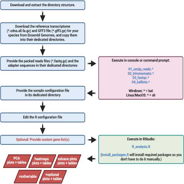
Workflow of the PlugNSeq pipeline
After downloading and extracting the provided directory structure, the user only needs to follow four basic steps in the protocol (Figure 1). First, the user copies the required reference transcriptome, GFF3, RNA-Seq reads and adapter sequence files into dedicated folders. Then, four consecutive scripts are executed by the user. After the scripts have been successfully executed, the user edits the provided and partly newly created sample configuration file (required) and R configuration file (optional), and saves them in their dedicated folder. Finally, the provided R script is run by the user in RStudio. That's it. The results include PCA scores plots with accompanying tables, a volcano plot for each pairwise comparison, a main horizontally and vertically clustered heatmap (based on z-scores of the group means) with all genes that were significantly regulated in at least one of the pairwise comparisons, including the accompanying table. Additionally, a heatmap of fold-changes in the pairwise comparisons will be generated, which also comes with an accompanying table. Furthermore, the user receives the "mothertable", a spreadsheet that contains the locus and transcript ID's, annotations, all sample expression values and group mean expression values as well as corrected p-values, log2-fold-changes and regulation patterns of each gene for all pairwise comparisons performed. There will also be a heatmap of the replicate samples, allowing for quick assessment of sample quality. This heatmap has no accompanying table since it is only meant for visual inspection. Optionally, the user may provide custom gene lists before the R analysis starts, and then gets dedicated heatmaps for each of the provided gene lists, including the respective accompanying table. These heatmaps include ones that are created using z-scores of the group means, and ones that are created based on the fold-changes in all pairwise comparisons performed. All important heatmaps are created in two customizable three-step color palettes and in several sizes.
Figure 1. Detailed overview of the PlugNSeq pipeline workflow. The black arrows guide through the steps in the pipeline. Blue arrows point to results or outputs of a step. Red arrows indicate that something is used as an input for a subsequent step. Light blue boxes indicate steps that the user must perform. Pink boxes mark the shell (Linux or Mac OS) or batch scripts (Windows), that automatically do all the hard work of preprocessing the data, quality control, and pseudoalignment and quantification of the reads, once the data have been provided by the user according to the protocol and guidelines (blue boxes). The green box marks the R script that automatically creates all the basic graphs and tables in a most convenient way.


Image Attribution
Guidelines
The reference transcriptome file
We recommend downloading the reference transcriptome file from Ensembl Genomes. Files from Ensembl Genomes adhere to our naming convention. Ensembl Genomes offer two formats of the reference transcriptome files. You may either download a FASTA file (*.fa or *.fasta), or a gzip-compressed archive containing the FASTA file (*.fa.gz or *.fasta.gz). You may use either one of these two formats. The scripts will deal with them accordingly. If you decided to download the reference transcriptome from somewhere else, please make sure that the FASTA file has the file extension ".fa" or ".fasta", and that the file extension of a gzip-compressed file is ".fa.gz" or ".fasta.gz". This is required for the scripts to recognize them properly. For the best results, it is strongly recommended that the reference transcriptome file contains the cDNA sequences (CDS + 5'-UTR + 3'-UTR). These files are usually named "*.cdna.all.fa" or "*.cdna.all.fa.gz" (when gzip-compressed). If there is no such cDNA file, you may use the coding sequences (*.cds.all.fa or *.cds.all.fa.gz). Keep in mind that using CDS will reduce the alignment efficiency significantly, since reads that may align to 5' or 3'-UTR cannot be aligned.
The GFF3 file
We recommend downloading the GFF3 file from Ensembl Genomes. Files from Ensembl Genomes adhere to a certain naming scheme. Ensembl Genomes offer two formats of the GFF3 files. You may either download a GFF3 file (*.gff3), or a gzip-compressed archive containing the GFF3 file (*.gff3.gz). You may use either one of these two formats. The scripts will deal with them accordingly. Other file extensions such as ".gff" for uncompressed or ".gff.gz" for compressed files indicate a potentially incompatible file format and may lead to errors. We strongly recommend downloading the GFF3 file from the same resource as the reference transcriptome file. Retrieving them from different sources may lead to inconsistencies, which themselves may lead to errors during the final analysis in R. Downloading GFF3 or GFF files from resources other than Ensembl Genomes will very likely require adapting the respective entries in the file "configuration_r_analysis.R".
RNA-Seq reads files naming convention
RNA-Seq reads must contain reads in the FASTQ format and follow the Illumina file naming convention (Illumina, 2024). It is best to keep file names unchanged, as our scripts rely on this format. If files come from other platforms, rename them to fit the minimally required format below, which is a simplified version of the Illumina file naming convention.
Single-End vs. Paired-End Reads:
The distinction between single-end (SE) and paired-end (PE) reads is crucial, as they require different processing. Sequencing facilities typically deliver reads as compressed "*.fastq.gz" or "*.fq.gz" archives. Our shell scripts differentiate between SE and PE reads using specific naming patterns.
Single-end reads (SE):SE files use "_R1" as an identifier. "_R1" should appear either between <namePart1> and <namePart2> or directly after <namePart1> if <namePart2> is omitted. This applies to both compressed (*.gz) and uncompressed (*.fastq or *.fq) formats:
<namePart1>_R1<namePart2>.fastq.gz > compressed FASTQ
<namePart1>_R1.fastq.gz > compressed FASTQ, <namePart2> omitted
<namePart1>_R1<namePart2>.fq.gz > compressed FQ)
<namePart1>_R1.fastq.gz > compressed FQ, <namePart2> omitted
Paired-End Reads (PE):
PE files are identified by "_R1" for forward reads and "_R2" for reverse reads. The <namePart1> and <namePart2> (if applicable) must be identical in each pair. This applies to both compressed (*.gz) and uncompressed (*.fastq or *.fq) formats:
<namePart1>_R1<namePart2>.fastq.gz > 1st of pair, FASTQ
<namePart1>_R2<namePart2>.fastq.gz > 2nd of pair, FASTQ
<namePart1>_R1.fastq.gz > 1st of pair, FASTQ, <namePart2> omitted
<namePart1>_R2.fastq.gz > 2nd of pair, FASTQ, <namePart2> omitted
<namePart1>_R1<namePart2>.fq.gz > 1st of pair, FQ
<namePart1>_R2<namePart2>.fq.gz > 2nd of pair, FQ
<namePart1>_R1.fq.gz > 1st of pair, FQ, <namePart2> omitted
<namePart1>_R2.fq.gz > 2nd of pair, FQ, <namePart2> omitted
Key Points:
- Single-End Reads: Each sample/replicate has one file containing "_R1".
- Paired-End Reads: Each sample/replicate has a pair of files — one with "_R1" (forward) and the other with "_R2" (reverse).
- "_R1" and "_R2" must appear exactly once in the file name and only in the specified positions.
- <namePart1> and/or <namePart2> (if used) uniquely identifies the sample/replicate. For paired-end reads, both <namePart1> and/or <namePart2> (if used) must match within each file pair but also be unique to that pair.
This streamlined format ensures compatibility with our scripts while maintaining clarity between single-end and paired-end data. Reads files generated by any Illumina HiSeq platform should match this pattern by default.
The sample configuration file
The table "configuration_samples.tsv" is initially not available. It is created automatically at the end of pseudoalignment and quantification of the reads. The file is located in the subdirectory "./R_analysis/configuration" (Linux or Mac OS) or "\R_analysis\configuration" (Windows). The file is required to define the factors, factor levels, and replicate numbers for your experiment. The file is pre-filled with the file names of the respective quantification TSV files, that match the original reads file names but with the file extension "*.tsv". In the column names shown below, "n" represents the number of the respective factor. Up to 4 different factors are possible. Examples of fully filled files for different numbers of factors are included in the subdirectory "./R_analysis/configuration/example_configuration_tsv_files" (Linux or Mac OS) or "\R_analysis\configuration\example_configuration_tsv_files" (Windows).
The File Name Column (file):
This is the first (leftmost) column. It is pre-filled with the quantification TSV file names, which are named according to the original reads files. These file names must not be changed.
Factor Columns (factor_n):
Each "factor_n" column represents a factor in your experiment and must be filled with the name of the factor (e.g., "organ", "genotype", "fertilizer", "temperature"). This value must remain identical in all rows of the respective column.
Factor Level Columns (factor_n_level):
Fill the "factor_n_level" column with the detailed description of the factor level (e.g., "old leaf" or "young leaf" if the factor is "organ", or "wildtype", "mutant 1" or "mutant 2" if the factor is "genotype" etc.) for each row. This should correspond to the sample indicated by the "file" column.
Shortened Factor Levels (factor_n_level_short):
Enter a short abbreviation for each factor level in the "factor_n_level_short" column (e.g., "ol" for "old leaf", or "yl" for "young leaf", "wt" for "wildtype" or "m1" for "mutant 1" etc.). This abbreviation should match the corresponding factor level. It must start with a letter ([a-z][A-Z]) and may contain numbers ([0-9]), but no space and no special characters.
Factor Level Priority (factor_n_level_priority):
Assign a priority rank (e.g., "1" or "2") for each unique factor level in the "factor_n_level_priority" column. This priority will determine the order of pairwise comparisons (e.g., 2 vs. 1 instead of 1 vs. 2). It is enough (and best) to enter the priority rank only once at an occurrence of the respective factor level, but each factor level must have a priority rank assigned.
The Column for Replicate Numbers (replicate_number):
This is the last (rightmost) column. Enter a replicate number (e.g., "1," "2," "3") in the "replicate_number" column for every row. This is required for all samples/files.
Unused Factor Columns:
If your experiment does not include all four factors, leave the unused factor columns (and their corresponding level, short, and priority columns) empty. Only fill the factor columns where "n" is smaller or equal to the actual number of factors. Please find four example configuration TSV files for different numbers of factors in the subdirectory "./R_analysis/configuration/example_configuration_tsv_files/".
The file can be opened with spreadsheet software such as Microsoft™ Excel or LibreOfficeThe file name must be in all small letters configuration_samples.tsv" (unchanged original TSV file format), "configuration_samples.xlsx" (Microsoft™ Excel) or "configuration_samples.ods" (LibreOffice Calc). The file name must be in all small letters. The analyzing script can read all three formats.
The R configuration file
In addition to the sample configuration file, file that is automatically generated at the end of the quantification step (configuration_samples.tsv), the subdirectory "./R_analysis/configuration/" (Linux or Mac OS) or "\R_analysis\configuration" (Windows) also contains a file to configure the statistical analysis in R. The file is named "configuration_r_analysis.R". It can be edited directly in RStudio. The following parameters can be changed:
- adjust_methodThis is the p-value correction method. Here, the user may enter "bonferroni" (FWER by Bonferroni) or "BH" (FDR by Benjamini Hochberg). The value must be assigned to one of the available options and must not be empty. The default entry is "bonferroni".
- log2fc_thresholdThis is the log2-transformed fold-change threshold. Only genes that are differentially regulated with a fold-change higher than this threshold may be considered regulated in conjunction with a significant corrected p-value. The user may enter any positive value larger or equal to 0 (zero). Entering 0 (zero) means that the log2-fold-change threshold is ignored. 1 means that only genes with a fold-change of two-fold or higher are considered regulated in conjunction with the p-value threshold. 0.5849625 means a fold-change of 1.5-fold or higher. The default entry is 0.5840625 (1.5-fold or higher).
- q_thresholdThis is the corrected p-value threshold. It may be set to more stringent values such as 0.01, which is particularly recommended when the log2-fold-change threshold (see above) is ignored, or when very stringent analysis is required. The default entry is 0.05.
- comparisonsThis denominates whether all possible pairwise comparisons (really all the possible combinations) or only the "good" ones, where the two groups differ in exactly one factor level, will be performed.
- clustersThis is the number of vertical gene clusters that are created in the main heatmap. It can be set to any value between 2 and 15. Please keep in mind that this number must be smaller than the total number of significantly regulated genes. If it is larger than 15 or larger than the number of regulated genes, it will automatically be set to the nearest value that fits.
- compressionThis value is used to limit the maximum (and minimum) of the z-scores in the color palette of a heatmap of samples or group means (main heatmap, heatmap of custom genes and heatmap of replicate samples). 1 means that the original maximum and minimum is used (whichever has the higher absolute value) as the positive and negative borders, where the color reaches its maximum saturation and above which the color does not change anymore. If the colors in the heatmaps are too faint, there are probably a few very high or very low z-scores that stretch the range so much that the majority of the values are very close to zero (relative to the available range). In this case you may increase this value. If the colors are too saturated, you may decrease this value. You must enter at least the value 1. The standard value is 2. Values with decimal points such as 1.2 or 2.7 are also possible. The range in the color palette is limited to the maximum or minimum of the z-scores (whichever has the higher absolute value) divided by this number. The legend at the extreme values says: ">=a" and "<=b" (a = upper limit, b = lower limit).
- compression2This is the same as "compression" but for heatmaps of the comparisons there the range of log2-fold-changes is limited the same way as the z-scores by "compression" in the other heatmaps. So the user is able to adjust the color saturation in these two types of heatmaps separately. The standard value is 1.5.
- color_paletteThis is the three-step color palette for heatmaps. You may replace the existing color values by your own color values. Standard is blue-black-yellow (low-medium-high).
- color_palette2This is the alternative three-step color palette for heatmaps. You may replace the existing color values by your own color values. Standard of the alternative color palette is red-black-green (low-medium-high).
- gff3_transcript_idIn GFF3 files from Ensembl this is "transcript_id" (default). It's the attribute that contains the transcript ID in lines where type is "mRNA"
- gff3_parentIn GFF3 files from Ensembl this is "Parent" (default). It's the attribute that contains the locus ID in lines where type is "mRNA".
- gene_idIn GFF3 files from Ensembl this is "gene_id" (default). It's the attribute name that contains the gene identifier / locus ID (e.g. At3g12900 or Os01g0100900 or ENSG00000186092) in lines where type is "gene", if available.
- gene_symbolIn GFF3 files from Ensembl this is "Name" (default). It's the attribute that contains the gene symbol(s) (e.g. AtS8H or OsSPL1 or OR4F5) in lines where type is "gene", if available.
- gene_descriptionIn GFF3 files from Ensembl this is "description" (default). It's the attribute that contains the gene description in lines where type is "gene", if available.
Note
If no descriptions or gene symbols are available in your GFF3 file, please leave as is. The respective fields will then stay empty and can be filled manually later. Alternatively, the user can provide their own annotations.
Note
If you download the GFF3 file from Ensembl Genomes, no changes are required. Otherwise, it is up to the user to find the right attributes and names in their particular GFF3 file and to enter them correctly here. Some providers provide GFF files (instead of GFF3) separated into "locus", "transcripts" and more. Then, it is best to just paste them together, remove possible duplicate rows, save the bigger file as GFF3 and search for the respective attributes.
[Optional] Custom lists of genes of interest
The user may provide custom lists of genes as "my_gene_lists.tsv" (unchanged original tab-separated values format), "my_gene_lists.xlsx" (Microroft™ Excel spreadsheet format) or "my_gene_lists.ods" (LibreOffice Calc spreadsheet format). The file(s) must be put into the directory "./R_analysis/my_gene_lists" (Linux or Mac OS) or "\R_analysis\my_gene_lists" (Windows). Each column represents a separate list. For each list there will be a separate heatmap including the accompanying table. The 1st row must contain the name of the list (Figure 2). You may choose the names freely. The 2nd row must contain the number of clusters for the respective list (column), into which the genes will be clustered in that particular heatmap (Figure 2). The number of clusters must be smaller than or equal to the number of genes in the heatmap. The different lists (columns) may have different numbers of entries. Only locus identifiers are accepted. The analysis is case sensitive. Therefore, please make sure that the letter case matches between the reference transcriptome and GFF3 file, and the provided list(s). Irrespective of the chosen file format, the name of the file must be in all small letters. If there are several such files with different formats, the anayzing script will first read the *.xlsx file (if there is one) and ignore the others, then the *.osd file (if there is one) and ignore the *.tsv file, and finally read the *.tsv file (if there is one) if there is none of the other formats.
| A | B | C | |
| my list 1 | my list 2 | ||
| 4 | 12 | ||
| At3g07720 | At5g12470 | ||
| At3g12900 | At3g06880 | ||
| At3g13610 | At2g36750 | ||
| ... | ... |
Figure 2. Example spreadsheet view of two custom gene lists. Each column is a separate list. Every column can hold as little or as many genes as desired. The first row must contain the list name(s) and the second row must contain the desired number of gene clusters in that particular heatmap. The actual lists begin at row 3. Only gene identifiers are allowed here. The letter case must match the case used in the reference transcriptome or GFF3 file.
[Optional] Own annotations
The user may provide their own annotations in form of locus ID, symbol and description. This is done by providing a spreadsheet file where the 1st column has the header "locus_id" (without quotes) in the field A1, the second column has the header "my_symbol" (without quotes) in B1, and the second column has the header "my_description" in C1. Below these headers in row 1, the user may put the locus identifiers in column A, the respective symbols in column B and the matching descriptions in column C.
| A | B | C | |
| locus_id | my_symbol | my_description | |
| AT3G53260 | PAL2 | Encodes phenylalanine lyase. Arabidopsis has four ... | |
| AT1G28680 | COSY | Catalyses trans-cis isomerization and lactonization in ... | |
| At3g12900 | S8H | S8H hydroxylates scopoletin to generate fraxetin ... | |
| At3g13610 | F6'H1 | Encodes a Fe(II)- and 2-oxoglutarate-dependent ... | |
| ... | ... | ... |
Figure 3. Example spreadsheet view of annotations as they can be provided with a spreadsheet file. The first row must contain the column headers "locus_id", "my_symbol" and "my_description" (without quotes) and the rest of the rows contain the annotations. In the column "locus_id" only gene identifiers are allowed. The letter case should match the case used in the reference transcriptome or GFF3 file.
The directory structure
In the Attachments we provide a predefined directory structure to streamline the management of the user’s experimental data (Figure 4). The central directory, "PlugNSeq", encompasses various specialized subdirectories for different stages of data processing. Initially, compressed "*.fastq.gz" files are stored in "PlugNSeq/04_user_packed_reads" (Linux or Mac OS) or "PlugNSeq\04_user_packed_reads" (Windows), and upon decompression, the resulting ".fastq" files will be relocated to "PlugNSeq/unpacked_reads" (Linux or Mac OS) or "PlugNSeq\unpacked_reads" (Windows). Following this, the reads trimmed by Trimmomatic are placed in "PlugNSeq/trimmed_reads" (Linux or Mac OS) or "PlugNSeq\trimmed_reads" (Windows), while the outputs from FastQC and kallisto quantification are stored in "PlugNSeq/fastqc_output" (Linux or Mac OS) or "PlugNSeq\fastqc_output" (Windows), and "PlugNSeq/kallisto_output" (Linux or Mac OS) or "PlugNSeq\kallisto_output" (Windows), respectively.
These specific output subdirectories are pre-included within the provided structure and can be emptied as the workflow begins; the necessary scripts are designed to recreate them if needed. It is important to maintain the integrity of the remaining directories with their original naming, and their contents, for the scripts to operate correctly. However, the "PlugNSeq" parent directory can be renamed without impacting script functionality. We suggest that you leave the directory names untouched. Please see the README file in most of the directories that explains their purpose. Some directories contain subdirectories named "/out_of_sight" (Linux or Mac OS) or "\out_of_sight" (Windows). These may serve as storage for files that can be re-used later. So you have them on hand when they are needed. The scripts will not search in these subdirectories. Files therein will be ignored and remain untouched.
Furthermore, the "R_analysis" directory is set up to house the R script and related files across its subdirectories, allocated for user-provided data or data that are generated during pre-processing and quantification. The actual results of the R analysis, including a detailed spreadsheet, the "mothertable", plots, and additional tables that correlate with the plots, will be saved in a newly subdirectory named “PlugNSeq/R_analysis/r_results_<date>_<time>_<parameters>” (forward slash as directory divider in Linux or Mac OS) or “PlugNSeq\R_analysis\r_results_<date>_<time>_<parameters>” (backslash as directory divider in Windows). Each time, the R script is executed, a new unique results subdirectory will be created. This organizational approach is aimed at ensuring a smooth and orderly process for handling and analyzing the user’s experimental data, and keeping track of the parameters used in each particular execution of the R script.
Figure 4. The PlugNSeq folder structure, partially collapsed tree view with the major steps indicated. 1. The files provided by the user (reference transcriptome file, GFF3 file, the packed reads, and the adapter sequences) are put into their respective directories. This ensures that the shell/batch scripts can find the required data and process them properly. 2. The four shell (Linux/Mac OS) or batch scripts (Windows) are executed sequentially. This includes unpacking the packed reads, trimming the unpacked reads, quality control of the trimmed reads, and finally, quantification of the reads. 3. The sample configuration file (required) and the R configuration file (optional) are edited/completed according to the guidelines. This ensures that the R script is given all the required information to perform the statistical analyses properly. 4. The R script "R_analysis.R" is executed in RStudio. 5. The results are stored in a newly created subdirectory inside the "R_analysis" directory. If the R script is to be run for the very first time, another script "install_packages.R", which can be found in the "helper" subdirectory, can be run beforehand. It will install all the required packages used in "R_analysis.R".
Materials
Required skills
This protocol requires only basic knowledge in Linux, Mac OS or Windows by the user. The user should be able to install software from the available repositories, or from a downloaded installer, and know how to open and run an R script in RStudio. Under Linux and Mac OS, the user should be able to use a file manager, and know the basics of working with the terminal: How to navigate to a certain folder, how to move, copy and rename files and directories, and possibly how to make a file executable. Under Windows, the user should only know how to copy, move and delete files. In all cases the user should be able to edit a spreadsheet using software such as LibreOffice or Microsoft™ Excel. Everything else is described in the protocol.
Required directory structure
Data is organized in a specific directory structure. The user does not need to create the directory structure and files therein, since everything is provided with the files in the Attachments.
Required hardware
This protocol will run on any modern computer or workstation with just enough memory. Depending on the speed and number of available CPU cores/threads, the duration of the single steps may vary widely, but any CPU with 4+ cores/threads will work. For very large experiments (e.g. 4 factors with 2-3 levels each), we recommend at least 16 GB or better 32 GB of memory (RAM). Smaller experiments (e.g. 2 factors with 2-3 levels each) may run with as little as 8 GB of RAM. The storage space must exceed the amount of data required for this pipeline. The total amount of required free space can be calculated by multiplying the total size of your packed reads by 10. If the total size of your packed reads is 30 GB, please make sure to have at least 300 GB and a bit more of free drive space on the partition, on which you perform this protocol.
Required software
This protocol is compatible with Mac OS, Linux and Windows. For trimming, quality control, pseudoalignment, and quantification, Trimmomatic version 0.39 (Bolger et al., 2014), FastQC version 0.11.9 (Andrews, 2017) and kallisto version 0.46.1 (Bray et al., 2016) are utilized in the protocol. These tools were retrieved from the official resources. RStudio is used to perform the statistical evaluation and visual representation of the data. It was installed from the package downloaded from the developers' website, or via relevant repositories. Usually, R is automatically installed as a dependency of RStudio. However, in some Linux distributions, Mac OS and Windows, R must be installed separately from RStudio. Notably, Trimmomatic, FastQC, and kallisto do not require separate installations as the binary files are provided (along with the respective license information) within the directory structure. This ensures the functionality of the scripts even if the system-wide commands cannot be determined or if the software is not installed at all. Thus, installation of Trimmomatic, FastQC, and kallisto is unnecessary and will not be covered. Besides Rstudio, a number of R packages will be utilized. These are installed within R, and they include the cran packages remotes, stats, purrr, magick, writexl, tidyverse, rstudioapi, gtools, ggplot2, ggpubr, cowplot, ggrepel, rgl, liver, pheatmap and RColorBrewer, as well as the Bioconductor packages rtracklayer (Lawrence et al., 2009), limma (Ritchie et al., 2015), and edgeR (Robinson et al., 2010). Since some of the above software requires a Perl interpreter, Perl must be intsalled. In many Linux distributions and Mac OS versions, a system perl interpreter is usually pre-installed. In Mac OS, newer versions Perl can be installed manually. In Windows, a perl interpreter must be installed manually. Strawberry Perl (https://strawberryperl.com/) is a free and open source solution for Windows. In most Linux distributions, a Java Runtime Environment is pre-installed. In Mac OS and Windows, it must be installed manually with the respective installer file downloaded from java.com.
Note
There are many alternatives available. However, all programs and packages used in this protocol represent well-established and approved tools in the field of transcriptome analysis. Due to its ease of use, speed, and resource efficiency, kallisto was selected for pseudoalignment and quantification of the reads. It can perform the required operations on a standard, up-to-date PC. Additionally, local processing of the data was chosen because it does not require uploading critical research data to a third-party server, adhering to many institutions’ data privacy and security policies.
Training Data
We provide training data from a rice experiment (Kar, Mai et al., 2021) under https://doi.org/10.25838/d5p-70. On the linked page you will find 24 packed reads files. They are paired-end. If you want to check processing single-end reads, you may only use files with "R1" in the name. They will automatically be treated as single-end reads if the partner "R2" file is missing.
Troubleshooting
Safety warnings
Memory:
For small experiments, the protocol will run on a Laptop/PC with 8 GB of memory. Larger experiments may require 16 GB or more. I recommend at least 16 GB of memory whereas 32 GB is safe to use even with very large experiments. If you try and analyze an experiment that is large enough to use up all the available memory, the computer might crash. This may lead to loss of unsaved work. If in doubt, please save all unsaved work and close all unnecessary software before executing the protocol. The preprocessing scripts will ask you for the number of threads to use or the number of files to be processed in parallel. This way you can restrict effectively the amount of memory used.
Storage space:
Many new files will be generated during the process. Exceeding the available storage space may make your storage device very slow or even result in loss of data, particularly with SSD's. Therefore, please make sure that there is enough space on the storage device, with which you are going to execute this protocol. You may roughly calculate the expected total amount of required storage space by multiplying the total size of your packed reads with 10-12. Hence, if your reads files are 30 GB in size, make sure to have at least 360 GB of free space on the partition where you execute this protocol. There are some options to save storage space, which will be explained with the respective steps in the protocol.
SSD drives:
If lots of data are written and deleted again from an SSD drive, the drive might get very slow or even temporarily unusable. This may happen if the "TRIM" command is not executed. Usually, this happens once a week. Should you encounter this problem, you may wait until the problem automatically disappears (the operating system trims the drive, after which everything is okay again), or invoke trimming manually to resolve the problem immediately. If you plan to perform several analyses within only a few days with writing and deleting lots of data, it is recommended to invoke trimming the SSD manually right after freeing up space for another analysis and after emptying the recycle bin (don't forget to do this) but before copying new data to the drive.
Before start
Make sure that the following is readily available:
- The packed reads files of your RNA-Seq experiment (*.fastq.gz or *.fq.gz)
- The adapter sequence(s) used for library preparation (if not provided, ask your sequencing facility)
- Information on which SE file or pair of PE files represent which sample/replicate
- Information on the experimental setup (factors and factor levels)
Note
To enable the R scripts to recognize your samples and replicates, and to process the data correctly, you will have to provide information on the experimental setup in form of a configuration file (Microsoft Excel spreadsheet). After preprocessing the reads and quantification of the transcripts, a pre-filled template file will be generated, that only has to be edited by the user. There are also fully filled example files for different cases. More information on that is provided with the respective steps in the protocol.
Make sure that your notebook/PC/workstation has enough storage space to hold all the RNA-Seq reads, which can easily exceed 1 TB in very large experiments. If necessary, free up enough storage space to hold the data.
It is highly recommended to check the packed reads files for potential errors that may have occurred during the file transfer. This is usually done using checksums. If you are not given any checksums, please ask your sequencing facility.
Install a perl interpreter:
In the most common Linux distributions and Mac OS, a system Perl interpreter is pre-installed by default. In Mac OS a newer version of perl can be installed manually. In Windows, a perl interpreter must be installed manually. To install perl on Mac OS, please follow the instuctions on Learn Perl. To install perl on Windows, please download the MSI installer from https://strawberryperl.com/ and install Strawberry Perl for Windows.
Install a java runtime environment:
A system Java interpreter comes preinstalled with Mac OS older than 10.7. and in most Linux distros. In newer Mac OS versions (>10.7) and Windows, a Java Runtime Environment (JRE) must be installed manually. To install JRE on Mac OS or Windows, please download the respective installer from java.com.
Install R:
If R has not been installed yet, please install R from the repositories, or from an installation file (depending on your operating system) downloaded from the developers' website (https://www.r-project.org/).
Note
In Linux, R is automatically installed as a dependency when installing RStudio from supported repositories (see below). Therefore, separate installation of R is often not required in Linux.
Install RStudio:
If RStudio has not been installed yet, please install RStudio from the repositories, or from an installation file (depending on your operating system) downloaded from the developers' website (https://posit.co/download/rstudio-desktop/).
Note
If installed from the official repositories or other supported repositories in Linux, the dependency R is usually installed automatically with RStudio. If installed from a downloaded installation file, you might also have to install R manually (see above).
Download the required directory structure:
If you are working under a Windows operating system, download the file "PlugNSeq_win.zip". If you are working under Linux or Mac OS, download the file "PlugNSeq_linux_mac.tar.gz". See the Attachments to download the files. These packed files contain the complete required directory structure for your operating system, including the necessary tools, bash (Linux or Mac OS) and batch scripts (Windows) and R scripts.
Download the reference transcriptome file:
Download the reference transcriptome file for your organism of interest from Ensembl Genomes (recommended) or from another resource.
Note
The reference transcriptome files from Ensembl Genomes containing the cDNA sequences usually end with ".fa", ".fasta", ".fa.gz", or ".fasta.gz". Our scripts can work with all of these formats, so we recommend downloading the smaller compressed file (*.gz). If cDNA sequences are not provided, you may use the coding sequences (CDS) instead. Files containing the CDS from Ensembl Genomes usually also end with ".fa", ".fasta", ".fa.gz", or ".fasta.gz". Here, you may also use both formats. Keep in mind that using CDS instead of cDNA sequences will reduce the alignment efficiency.
If you choose to download the reference transcriptome from another resource, the file names might not end with ".fa", ".fasta", ".fa.gz", or ".fasta.gz". If so, please rename the file extension so that a FASTA file ends with ".fa" or ".fasta", or a gzip-compressed FASTA file ends with ".fa.gz" or ".fasta.gz". If in doubt, please extract the FASTA file from the archive. If necessary, rename the file extension of the extracted FASTA file to ".fa" or ".fasta". See Guidelines ("Naming convention for the reference transcriptome file").
Download the GFF3 file:
Download the GFF3 file for your organism of interest from Ensembl Genomes (recommended) or from another resource.
Note
The annotation files from Ensembl Genomes usually end with ".gff3.gz". Hence, they are gzip-compressed archives containing the GFF3 file. You may use them as they are, or extract the GFF3 file and use the extracted file. However, the compressed file must have the file extension ".gff3.gz", and the extracted GFF3 file must have the file extension ".gff3". Please see Guidelines ("Naming convention for the GFF3 file"). The annotation file must be downloaded from the same resource as the transcriptome file. If you decide to download the reference transcriptome from another resource, you must download the GFF3 file from that same resource.
Download the required directory structure
If you are working under a Windows operating system, download the file "PlugNSeq_win.zip". If you are working under Linux or Mac OS, download the file "PlugNSeq_linux_mac.tar.gz". See "Attachments" to download the directory structure. From here on, please select and follow one of the cases below ("Linux or Mac OS", or "Windows"), according to your operating system.
Linux or Mac OS13 steps
Prepare the required directory structure
Copy or move the downloaded file (PlugNSeq_linux_mac.tar.gz) to the destination drive and directory. Open a terminal, navigate to the directory where "PlugNSeq_linux_mac.tar.gz" is stored, and extract the tarball by executing the following command:
Command
new command name
Expected result
In the current directory, this will create a new directory named "PlugNSeq", which contains all the required shell scripts, subdirectories and files. Please check the new directory "PlugNSeq". In the following, we will refer to possible subdirectories as subdirectories of "PlugNSeq".
Note
The partition, to which the tarball is extracted, should be formatted using a file system that can store permission bits, such as ext3 or ext4 (Linux), or APFS or HFS+ (Mac). Here, all scripts and software will be executable if the folder structure is extracted with the above command. On NTFS-formatted partitions, the scripts may have to be made executable manually. Upon successful decompression, the original file "PlugNSeq_linux_mac.tar.gz" may be deleted since it is not needed anymore. However, you may want to keep a copy in case you want to setup a new experiment.
Copy or move the required files to the respective directories
- Copy the downloaded reference transcriptome file into the directory "./01_user_transcriptome_file".
- Copy the downloaded GFF3 file into the directory "./02_user_gff3_file".
- Copy your compressed reads files to the directory "./03_user_packed_reads".
Note
See Guidelines and Before starting.
Provide the adapter sequence(s)
Edit either the file "my_se_adapters.fa" (single-end), or "my_pe_adapters.fa" (paired-end) in the directory "./04_user_adapters", depending on your type of reads. Remove unused adapter sequences that are already stored there, and add your own adapter sequence(s) in FASTA format. Save the file and close the editor.
In the following example example, the adapter sequences that were used in your RNA-Seq are "ACGTACGTACGTACGTACGTACGTACGT" and "TGACTGACTGACTGACTGACTGACTGAC", and you name them "My Adapter 1" and "My Adapter 2":
>My Adapter 1
ACGTACGTACGTACGTACGTACGTACGT
>My Adapter 2
TGACTGACTGACTGACTGACTGACTGAC
Preprocessing the Data
Decompression of the reads
To decompress the packed reads from the archives you provided, open a terminal, navigate to "PlugNSeq" and execute the shell script "01_unzip_reads.sh" by entering the command:
Command
new command name
Expected result
This will extract the packed reads from "./03_user_packed_reads" into "./unpacked_reads".
Note
This step is optional. You may skip it and start with the next step instead. If you start with the next step, the scripts will use the packed reads to perform the subsequent steps. This will save storage space but it will also take considerably more time.
Please keep in mind that the unpacked reads will take ca. 3 to 4 times as much space as the packed reads. Make sure that there is enough free space on your storage device.
Quality and adapter trimming
To start quality and adapter trimming, open a terminal, navigate to "PlugNSeq" and execute the shell script "02_trimmomatic.sh" by entering the command:
Command
new command name
The terminal then asks the user to enter an integer number of threads to be used. By default (if you enter no digits and just hit [Enter]) the script will use half the number of available threads.
Expected result
The trimmed reads (*.fastq or *.fastq.gz) will be stored in the "./trimmed_reads" subdirectory using the input file names with prefixes: "trimmed_paired_" for paired-end reads, "trimmed_unpaired_" for unmatched paired-end reads, or "trimmed_single_" for single end reads.
Note
Utilizing standard Trimmomatic parameters, the script checks for *.fastq files in "./unpacked_reads"; if found, they serve as input for quality and adapter trimming. Otherwise, it uses the compressed *.fq.gz or *.fastq.gz files from "./03_user_packed_reads". The output format of the trimmed reads matches the input format: *.fastq input files will result in *.fastq output files, and compressed *.fastq.gz or *.fq.gz input files will result in compressed *.fastq.gz output files.
Quality control of the trimmed reads
To assess the quality of the trimmed reads by executing the script "03_fastqc.sh", open a terminal, navigate to "PlugNSeq" and run the command:
Command
new command name
The terminal then asks the user to enter an integer number of reads files to be processed in parallel. By default (if you enter no digits and just hit [Enter]) the script will use half the number of available threads.
Expected result
This step, using FastQC, will generate HTML reports, which will be stored in separate subdirectories in the directory "./fastqc_output". The subdirectories are named according to the analyzed FASTQ files' names. For each FASTQ file (uncompressed or compressed) a report will be generated.
Note
With these reports, the user decides whether the reads' quality is good enough for further analyses. Running the script on packed trimmed reads (*.gz) will take significantly longer than with unpacked trimmed reads. The results must be looked at under all circumstances since bad quality reads and artifacts may strongly influence the results of the later steps such as alignment and quantification. For more information on FastQC results, please visit the author’s web site (https://www.bioinformatics.babraham.ac.uk/projects/fastqc).
Pseudoalignment and quantification of the reads
To build the index, pseudoalign the reads and quantify the transcripts, execute the script "04_kallisto.sh". Open a terminal, navigate to "PlugNSeq" and enter the command:
Command
new command name
Expected result
There will be a new file called "kallistoIndex" in the subdirectory "./kallisto_output". That is the index created using the reference transcriptome file by kallisto for pseudoalignment. Furthermore, there will be new subdirectories within "./kallisto_output", which will contain the quantification files as "abundance.tsv". Another new subdirectory "./all_tsv_files_renamed" will be created, which contains renamed versions of all the new "abundance.tsv" files according to the original file name(s). This makes it easy to match each quantification file with the original reads file(s). A copy of the renamed quantification files will also be stored in the subdirectory "./R_analysis/tsv_files", where they are required for further analysis. Furthermore a new file "configuration_samples.tsv" will be stored in the subdirecory "./R_analysis/configuration".
Note
The subdirectories containing the quantification files (abundance.tsv) are named according to the corresponding trimmed reads files. With single-end reads the subdirectories' names will match the names of the respective reads files (without file extension). With paired-end reads, one pair of files will result in a single quantification result. Therefore, the respective subdirectories' names will also match the file names of the pair of input files (without file extension) with the exception that "_R1" and "_R2" (the indicators for forward and reverse reads) are replaced by "_RX" in the respective subdirectory name. The new file "configuration_samples.tsv", which can now be found in the subdirecory "./R_analysis/configuration", is a pre-filled TSV (tab-separated values) file that must be completed by the user. It can easily be edited using spreadsheet software such as LibreOffice.
Preparations for Statistical Analysis in R
Edit the sample configuration file
The new table "configuration_samples.tsv", which is automatically created in the previous step, is used to define the factors, factor levels, and replicate numbers for your experiment. It is stored in the subdirectory "./R_analysis/configuration". Fill the file according to the Guidelines.
Note
Ensure that the table is fully filled out, with no missing values in the relevant columns for your experiment. Double-check that each unique factor level has a priority assigned. It is best to right-click the file name and then select "Open with..." > "<software>". After finishing the edits using, just click "File" > "Save" to save the edits without changing the file format. The user may also save the file as "configuration_samples.xlsx" (Microsoft™ Excel) or "configuration_sample.ods" (LibreOffice Calc). Example files with different numbers of factors can be found in "./R_analysis/configuration/example_configuration_tsv_files".
[Optional] Edit the R configuration file
In addition to the previously mentioned sample configuration file, file that is automatically generated at the end of the quantification step (configuration_samples.tsv), the subdirectory "./R_analysis/configuration" also contains a file to configure the statistical analysis in R. The file is named "configuration_r_analysis.R". It can be edited directly in RStudio. The file is pre-filled with standard parameters. The p-value correction method is "bonferroni", the corrected p-value threshold is 0.05, and the log2-fold-change threshold is 0.5849625 (1.5 or higher fold-change). The number of clusters for the heatmap is set to 15. You may leave it as is or change to your preferences.
- "adjust_method" values (p-value correction methods) may be "bonferroni" (FWER by Bonferroni) or "BH" (FDR by Benjamini Hochberg).
- "log2fc_threshold" values may be any log2-transformed fold-change. 0 (zero) means that no fold-change threshold is set. 1 means a fold-change of 2 or higher. 0.5849625 means a fold-change of 1.5 or higher.
- "q_threshold" (corrected p-value threshold) may also be set to more stringent values such as 0.01, which is particularly recommended when the log2-fold-change threshold is set very low or set to 0 (no fold-change threshold), or when very stringent analysis is required.
- "clusters" is the number of gene clusters that are created in the main heatmap. The default value is 15. It can be set to any value between 2 and 15. Please keep in mind that this number must be smaller than the total number of significantly regulated genes. Otherwise, it might cause errors.
Note
There are more lines that specify the attributes of the provided GFF3 file ("gff3_transcript_id", "gff3_parent", "gene_id", "gene_symbol", and "gene_description"). The attributes are explained in detail in the comments in that script. If you downloaded the GFF3 file from Ensembl Genomes, no changes are required. Otherwise, it is up to the user to find the right attributes and names in their particular GFF3 file and to enter them correctly here.
[Optional] Provide custom lists of genes of interest
The user may provide one or several custom lists of genes as "my_gene_lists.tsv" (unchanged original tab-separated values format), "my_gene_lists.xlsx" (Microroft™ Excel spreadsheet format) or "my_gene_lists.ods" (LibreOffice Calc spreadsheet format). Please provide the list(s) according to the Guidelines.
Note
Please enter only locus identifiers. The analysis is case sensitive, so please make sure that the letter cases match between the reference transcriptome and GFF3 file, and your provided list(s).
[Optional] Provide custom annotations
The user may provide a spreadsheet file named "my_annotations.xlsx" in the "my_annotations" subdirectory. Please find an example there (hidden in a subdirectory). The file may also be an ODS spreadsheet ("my annotations.ods") or a TSV file ("my_annotations.tsv"). The three columns must be "locus_id", "my_symbol" and "my_description" as described in the Guidelines.
Note
This may be useful if the GFF3 file has little or no annotations in form of gene symbols and gene descriptions.
Install the required R packages
The user may intall all the required packages manually. However, we provide an R script that does this for the user. The R script is called "install_packages.R", and it can be found in the directory "\R_analysis\r_script\helper". To install all the required R packages, open the script in RStudio and execute the script.
Note
As R sometimes "gets a hickup" (for lack of a better term) when installing many packages at once, the user might have to run the script several times until all the required packages are actually installed.
Final Statistical Analysis in R (Generation of Graphs and Tables)
Run the R script
Open the R script "R_analysis.R" in RStudio. The script can be found in "./R_analysis/r_script". To execute the script. This will perform all the basic statistical analyses.
Expected result
Upon running the script, a new subdirectory is created within "./R_analysis". Its name follows the pattern "r_<date>_<time>_<parameters>", where <date> and <time> represent the current timestamp, and <parameters> summarize the selected p-value correction method (e.g., Benjamini–Hochberg "BH" or Bonferroni "bonferroni") and the chosen minimum log2-fold-change threshold ("log2-fc"). This naming convention facilitates clear differentiation of results from different runs, even when identical parameters are used. The output subdirectories "mothertable", "heatmaps", "PCA", and "volcano_plots" contain the generated results.
PCA Analyses
- Scores plots (replicates and group means): PCA is performed separately on individual replicates and on group means. Score plots (PC2 vs. PC1 and PC3 vs. PC2) help assess replicate quality, detect outliers, and are publication-ready when based on group means.
- Gene loadings: For each PCA (replicates and means), gene loadings are analyzed. Genes' contributions to principal components are visualized in 3D scatter plots (PC1, PC2, PC3 axes). The 500 most influential genes are identified by geometric filtering (shrinking an ellipsoid around the data), highlighted in red in an interactive plot, and listed in an accompanying table.
- PCA of genes: PCA is also performed on genes, though plots are omitted due to density. A table of PCA scores is provided to support further analysis, such as identifying genes with distinct regulation patterns.
Mothertable
A comprehensive results table is generated in both TSV and Excel formats, containing:
- Locus identifiers
- Raw read counts
- TPM values per replicate and replicate group (means)
- Corrected p-values (FDR or FWER)
- Log2-fold-change values
- Regulation status (None, Up, Down) per comparison
- Annotations ("symbol", "description" from the GFF3 file
- Optional additional annotations ("my_symbol", "my_description")
Volcano Plots
Volcano plots are created for each pairwise comparison, visualizing fold-change versus significance. All required data are sourced from the mothertable.
Heatmaps
- The "main heatmap" (group means): Displays z-scores of all significantly regulated genes across replicate group means. Genes without significant regulation are excluded. Cluster numbers and annotations accompany the heatmap in a separate table. The number of clusters is configurable.
- Replicate sample heatmap: Displays the z-scores for individual replicate samples, enabling detection of outliers. This plot is intended for quality asessment and does not include a gene table.
- Comparison heatmap: Visualizes log2-fold-changes from all pairwise comparisons, with non-significant changes set to zero. Only significant differences contribute to clustering. A corresponding table is provided.
Optional: Custom Gene List Heatmaps
- Gene-list-specific heatmaps: If custom gene lists are provided, heatmaps are generated for each list, focusing on genes significantly regulated in at least one comparison. As with the main heatmap, accompanying tables are included, and cluster numbers can be specified per list.
- Comparison heatmaps for custom lists: Additional heatmaps visuaize log2-fold-changes for genes from each custom list, considering only significant changes.
Note
The heatmaps are created with two possible color schemes that can be customized in the R configuration file. Some heatmaps do not include gene identifiers since they would not be readable in a printed version. However, for some heatmaps there will be a "long" version trying hard to make individual gene identifiers readable in a very huge graph that is not meant for publication. The heatmaps for the custom gene lists will come in both versions (including and excluding locus identifiers). Both heatmaps derived from the custom gene lists will not only be available in different color schemes but also in different sizes and with different font sizes. Thus, the user can select the most suitable version when it comes to use a heatmap image for publication.
Note
Possible errors during the R analysis may be due to unavailable files, configuration files not filled correctly according to the guidelines, or (often!) due to typos in these files. Depending on the exact error message, please check these configuration files first, and then make sure that all the required files are available in the respective folders (TSV files in the "tsv_files" folder, the configuration files in the "configuration" folder and the GFF3 file in the "gff3_file" folder). The shell scripts for pre-processing and quantification of the reads are designed to give an error message if something goes wrong, indicating possible reasons for the error. In principle, possible reasons for errors are very similar those during the analysis in R.
Protocol references
Andrews, S. (2010). FastQC: a quality control tool for high throughput sequence data, https://github.com/s-andrews/FastQC.
Bolger, A. M., Lohse, M., & Usadel, B. (2014). Trimmomatic: a flexible trimmer for Illumina sequence data. Bioinformatics, 30(15), 2114-2120, https://doi.org/10.1093/bioinformatics/btu170.
Bray, N. L., Pimentel, H., Melsted, P., & Pachter, L. (2016). Near-optimal probabilistic RNA-seq quantification. Nature biotechnology, 34(5), 525-527, https://doi.org/10.1038/nbt.3519.
Kar, S., Mai, H. J., Khalouf, H., Ben Abdallah, H., Flachbart, S., Fink-Straube, C., ... & Bauer, P. (2021). Comparative transcriptomics of lowland rice varieties uncovers novel candidate genes for adaptive iron excess tolerance. Plant and Cell Physiology, 62(4), 624-640. https://doi.org/10.1093/pcp/pcab018.
Lawrence, M., Gentleman, R., & Carey, V. (2009). rtracklayer: an R package for interfacing with genome
browsers. Bioinformatics, 25(14), 1841.
Ritchie, M. E., Phipson, B., Wu, D., Hu, Y., Law, C. W., Shi, W., & Smyth, G. K. (2015). limma powers differential expression analyses for RNA-sequencing and microarray studies. Nucleic acids research, 43(7), e47-e47.
R Core Team. (2013). R: A language and environment for statistical computing. Foundation for Statistical Computing, Vienna, Austria. https://www.R-project.org/.
Robinson, M. D., McCarthy, D. J., & Smyth, G. K. (2010). edgeR: a Bioconductor package for differential expression analysis of digital gene expression data. Bioinformatics, 26(1), 139-140.
RStudio Team (2019). RStudio: Integrated Development for R. RStudio, Inc., Boston, MA URL, http://www.rstudio.com/.
Acknowledgements
I want to thank Dibin Baby, Mary Ngigi, Shahirina Khan, and Shishir Gupta for testing the PlugNSeq pipeline during various stages of development.