Mar 09, 2026
MorphoLogic: user guide for neuronal morphometrics and morphology-aware signal and puncta mapping
- Max Levian Sterling1,2,
- Sheersh Srivastava2,
- Naoki Kogo1,
- Richard van Wezel1,3,4,
- Nael Nadif Kasri2
- 1Donders Institute for Brain, Cognition, and Behaviour, Department of Neurobiology, Nijmegen, Netherlands;
- 2Radboud University Medical Center, Department of Human Genetics, Nijmegen, Netherlands;
- 3Techmed Center, University of Twente, Biomedical Signals and Systems, Enschede, Netherlands;
- 4OnePlanet Research Center, Radboud University, Nijmegen, Netherlands


External link: https://github.com/MaxLevianSterling/MorphoLogic
Protocol Citation: Max Levian Sterling, Sheersh Srivastava, Naoki Kogo, Richard van Wezel, Nael Nadif Kasri 2026. MorphoLogic: user guide for neuronal morphometrics and morphology-aware signal and puncta mapping. protocols.io https://dx.doi.org/10.17504/protocols.io.q26g77ppqgwz/v1
License: This is an open access protocol distributed under the terms of the Creative Commons Attribution License, which permits unrestricted use, distribution, and reproduction in any medium, provided the original author and source are credited
Protocol status: Working
contact: [email protected]
Created: January 14, 2026
Last Modified: March 09, 2026
Protocol Integer ID: 238631
Keywords: neuronal morphology, neuron morphology, dendritic morphology, dendrite, dendritic arbor, dendritic tree, neurite, neurite analysis, neuronal reconstruction, neuron reconstruction, morphology reconstruction, SWC, SWC file, SWC format, neuron tracing, neuronal tracing, dendrite tracing, digital reconstruction, morphometrics, morphometric analysis, morphological features, geometric analysis, branching, branch order, branching pattern, primary neurites, neurite segments, segment-level analysis, soma, soma ROI, somatic ROI, nuclear ROI, ROI, ROIs, ImageJ ROI, Fiji ROI, ROI set, microscopy, fluorescence microscopy, confocal microscopy, widefield microscopy, multi-channel TIFF, TIFF stack, image stack, immunofluorescence, MAP2, biocytin, dendritic marker, morphology channel, signal mapping, signal quantification, fluorescence intensity, intensity mapping, intensity profiling, signal density, density mapping, morphology-aware mapping, morphology-aware signal mapping, morphology-aware quantification, structure-function, synapse, synaptic, synapse density, synapse density mapping,
Funders Acknowledgements:
NWO NWA Scanner
Grant ID: 1518.22.136
Abstract
MorphoLogic extracts comprehensive neuronal morphometrics from 2D SWC reconstructions and can perform morphology-aware mapping to project concurrent microscopy signals or (synaptic) puncta onto reconstructed neurons. Beyond standard geometric and Sholl-style outputs, MorphoLogic provides a framework for mapping image-derived measurements onto the reconstructed tree and associating them with low-level architecture, supporting morphology-conditioned summaries such as signal or puncta density versus distance from soma, dendritic radius, branch order, or electrotonic distance.
Outputs include per-cell diagnostic visualizations and per-dataset aggregated CSV tables spanning segment-, branch-, neurite-, and cell-level summaries. The exported tables are structured for downstream group comparisons and stratified statistical profiling, with measurements aggregated across bins of morphological features and both absolute and normalized positional coordinates, and can readily be used to isolate subsets such as the largest neurite in post-hoc analyses.
Materials
Data inputs:
Morphology
- 2D neuronal reconstructions in SWC format (.swc) with non-zero radii are required. No additional tagging is necessary, but it is allowed. The first node (ID=1) should correspond to the soma (root), with all neurites connected to this node; the direct children of the root are treated as neurite starts. Each SWC file should contain a single cell.
- Soma ROI sets that define somatic regions per image (ImageJ/Fiji ROI format, e.g. ROI .zip containing multiple somas per image, or a single .roi for an individual soma).
Concurrent signal
- (Optional) Microscopy images in single-channel or multi-channel TIFF format (.tif/.tiff) for concurrent signals to be mapped (8-bit or 16-bit).
- (Optional, even when mapping a concurrent signal) Nuclear ROI sets that define nuclear regions per image (ImageJ/Fiji ROI format, e.g. ROI .zip containing multiple nuclei per image, or a single .roi for an individual nucleus). Nuclear regions often differ in intensity from the surrounding soma in the mapped signal and can be subtracted from the somatic region to obtain a more accurate estimate of somatic signal density.
Synapse puncta
- (Optional) Synapse puncta ROI sets that define synapse locations per image (ImageJ/Fiji ROI format, e.g. ROI .zip). Alternatively, the ROIs are also allowed be defined by a CSV file per image that has an 'X' and 'Y' column that describe the puncta locations in pixels (e.g., the standard SynBot output).
Hardware:
- Recommended for large datasets (thousands of cells): access to an HPC/cluster node.
Software:
- A command-line interface / terminal
- Python environment (see the step-by-step protocol or the GitHub repository for installation instructions)
- Fiji / ImageJ
- MorphoLogic
Troubleshooting
Problem
gui.py, ConfigError: Please choose a data directory.
Solution
In _build_config_from_form, set the GUI “Data directory” field to a valid folder path so the pipeline knows where to load inputs from.
Problem
gui.py, ConfigError: Directory does not exist: {directory}
Solution
In _build_config_from_form, pick a data directory path that exists on disk and is a directory (not a file).
Problem
gui.py, ConfigError: processing.extract_signal is enabled, but pathing.signal_channels is empty. Provide one or more channels (e.g. '1, 4') or disable extract_signal.
Solution
Either enter one or more signal channels in the GUI (e.g., 1, 4) or disable signal extraction.
Problem
gui.py, ConfigError: processing.extract_puncta is enabled, but pathing.puncta_roi_suffix is empty. Provide a suffix (e.g. '_puncta') or disable extract_puncta.
Solution
Provide a puncta ROI filename suffix in the GUI (e.g., _puncta) so puncta ROI files can be found, or disable puncta extraction.
Problem
gui.py, ConfigError: processing.deduct_nuclei is enabled, but pathing.nuclear_roi_suffix is empty. Provide a suffix (e.g. '_nuclei') or disable deduct_nuclei.
Solution
Provide a nuclear ROI filename suffix in the GUI (e.g., _nuclei) so nuclear ROI files can be found, or disable nuclear-signal deduction.
Problem
gui.py, ConfigError: visualization.signal.channel_names must have the same length as pathing.signal_channels.
Solution
Make visualization.signal.channel_names contain exactly one name per selected signal channel (same count/order).
Problem
gui.py, ConfigError: visualization.signal.channel_names contains empty names. Provide a non-empty name for each entry in pathing.signal_channels.
Solution
Replace any blank/whitespace channel name with a real non-empty label so plots don’t render missing titles/labels.
Problem
config.py, ConfigError: Config: 'pathing.directory' is empty. Set it in the Config defaults.
Solution
Set cfg.pathing.directory (in your config defaults or config file) to the data root directory before running.
Problem
config.py, DataNotFound: directory not found: {cfg.pathing.directory}
Solution
Update pathing.directory to an existing folder path (or create the directory) so it points to a real directory on disk.
Problem
config.py, ConfigError: Config: 'processing.extract_signal' is True but 'pathing.signal_channels' is empty. Either set signal_channels (e.g. (1, 4)) or disable extract_signal.
Solution
Provide one or more channels in pathing.signal_channels (e.g., (1, 4)) or disable processing.extract_signal.
Problem
config.py, ConfigError: Config: 'visualization.signal.channel_names' must have the same length as 'pathing.signal_channels'.
Solution
Ensure visualization.signal.channel_names has the same number of entries as pathing.signal_channels (one label per channel).
Problem
config.py, ConfigError: Config: 'visualization.signal.channel_names' contains empty names. Provide a non-empty name for each entry in 'pathing.signal_channels'.
Solution
Fill in any empty/whitespace names in visualization.signal.channel_names with non-empty labels.
Problem
config.py, ConfigError: Config: 'processing.extract_puncta' is True but 'pathing.puncta_roi_suffix' is empty. Either set puncta_roi_suffix (e.g. '_puncta') or disable extract_puncta.
Solution
Set pathing.puncta_roi_suffix (e.g., _puncta) so ROI files can be located, or disable processing.extract_puncta.
Problem
config.py, ConfigError: Config: 'processing.deduct_nuclei' is True but 'pathing.nuclear_roi_suffix' is empty. Either set nuclear_roi_suffix (e.g. '_nuclei') or disable deduct_nuclei.
Solution
Set pathing.nuclear_roi_suffix (e.g., _nuclei) so nuclear ROI files can be located, or disable processing.deduct_nuclei.
Problem
core.py, DataNotFound: No SWC/trace files under {self.cfg.pathing.directory}
Solution
Put .swc/trace files under cfg.pathing.directory (or fix the directory/patterns) so input discovery can find at least one trace.
Problem
core.py, DataNotFound: No processed PKLs under {processed_dir}
Solution
Run processing first (to create per-cell .pkl outputs) or point cfg.pathing.directory to a dataset that already has {cfg.pathing.directory}/Processed containing PKLs.
Problem
io.py, DataNotFound: Directory not found: {root}
Solution
Call discover_traces() with a root path that exists and is a directory (or create it).
Problem
io.py, DataNotFound: No base_suffix provided; cannot group '{criteria_extension}' files per image under: '{str(root)}'. Set base_suffix to a filename suffix such as '.traces' or '_8bit.tif'.
Solution
Pass a valid base_suffix (e.g., .traces or _8bit.tif) so discover_traces() can group criteria files by image stem.
Problem
io.py, DataNotFound: No '{criteria_extension}' files found under: '{str(root)}' using '{base_suffix}' as base suffix
Solution
Confirm the directory contains files matching the expected pattern (base files using base_suffix and corresponding criteria files using criteria_extension), or adjust base_suffix/criteria_extension to match your naming.
Problem
io.py, SWCParseError: Missing required SWC columns: {missing}
Solution
Ensure the SWC file loads into a DataFrame that includes all required columns (ID, Type, X, Y, Radius, Parent) with the correct headers.
Problem
io.py, SWCParseError: Column '{col}' contains non-numeric values. First bad row indices: {bad_rows}
Solution
Fix/clean the SWC so column '{col}' contains only numeric values (or adjust the exporter so it writes numbers).
Problem
io.py, SWCParseError: Column '{col}' contains non-integer values. First bad rows/values: {list(zip(bad_rows, bad_vals))}
Solution
For integer columns (ID/Type/Parent), ensure values are integers (no decimals); re-export or round/clean the SWC accordingly.
Problem
io.py, SWCParseError: SWC 'ID' must be positive. First bad row indices: {bad_rows}
Solution
Update the SWC so every ID is a positive integer (> 0); reindex nodes if needed.
Problem
io.py, SWCParseError: SWC 'Parent' should be -1 for root or a positive ID (0 is unusual/invalid). First bad row indices: {bad_rows}
Solution
Replace Parent==0 entries with the correct Parent ID, or -1 for the root node, to match SWC conventions.
Problem
io.py, SWCParseError: SWC contains dangling Parent references (not present in ID). First missing parent IDs: {dangling[:10]}
Solution
Ensure every Parent value (>0) refers to an existing ID in the same SWC; fix missing nodes or correct Parent pointers.
Problem
io.py, SWCParseError: SWC must satisfy ID > Parent for all non-root nodes (Parent != -1). First bad row indices and (ID, Parent) pairs: {list(zip(bad_rows, bad_pairs))}
Solution
Reorder/reindex nodes so each child has a larger ID than its parent (topologically sorted SWC), or re-export with correct ordering.
Problem
io.py, SWCParseError: SWC 'Radius' must be non-negative. First bad row indices: {bad_rows}
Solution
Remove/replace negative radius values with 0 or a valid positive radius (depending on your rules), and re-export.
Problem
io.py, SWCParseError: SWC 'Radius' must be > 0 for non-root nodes (Parent != -1). First bad row indices: {bad_rows}
Solution
Ensure all non-root nodes have Radius > 0 (fix measurement/export), since segments require a positive radius.
Problem
io.py, SWCParseError: Failed to read SWC '{filepath}': {e}
Solution
Fix the underlying parsing/IO issue reported in {e} (bad file path, malformed SWC, encoding issues, etc.) and re-run.
Problem
io.py, ValueError: CSV puncta file must contain X and Y columns: {f}
Solution
Add X and Y columns (case-insensitive is fine) to the puncta CSV so point ROIs can be constructed.
Problem
io.py, FileNotFoundError: No ROI file with suffix {suffix} for base {image_stem} in {folder}
Solution
Place an ROI file named like {image_stem}{suffix}... in {folder}, or change the configured suffix/image stem logic to match your filenames.
Problem
neurite.py, ValidationError: window_length must be >= 2 in {filename}; cannot fit regression with window_length=1.
Solution
Set radii_smoothing_window_length to 2 or higher (or disable radius smoothing) so linear regression is defined.
Problem
neurite.py, ValidationError: All original radii are 0 in {filename}; cannot compute padding/fit.
Solution
Fix the SWC so radii are non-zero (at least some nodes), or skip smoothing/segment construction steps that require meaningful radii.
Problem
neurite.py, ValueError: The line segment between node ID {node} and {neighbor} has no radius in {filepath}
Solution
Ensure both endpoints have Radius > 0 for all non-root segments (fix SWC radii), since frustum construction requires non-zero radii.
Problem
neurite.py, ValueError: No valid polygon could be formed from the points.
Solution
Fix degenerate geometry (overlapping points, near-zero segment length, clipped/collinear vertices, invalid radii) so the 4 frustum vertices can form a valid polygon; re-check SWC coordinates/radii and image bounds.
Problem
sholl.py, ValidationError: Sholl radii must start at 0 µm; got first radius {radii_um[0] if radii_um else None}.
Solution
Configure Sholl radii so the first radius is exactly 0 µm (e.g., range starting at 0) before running Sholl analysis.
Problem
sholl.py, ValidationError: {point_type.capitalize()} point ID {point_id} at {np.sqrt(dist_sq):.2f} µm is outside the Sholl range (max shell edge {max_r} µm).
Solution
Increase the maximum Sholl radius to cover the farthest nodes, or constrain/clean the reconstruction so branch/terminal points fall within the configured Sholl range.
Problem
soma.py, ValueError: Filename: {file}\nNo soma ROI contains ({px:.1f},{py:.1f}) px; available: {list((somatic_rois or {}).keys())}
Solution
Fix ROI placement or soma coordinate calibration so the SWC soma center (in px) lies inside exactly one soma ROI (or provide the correct soma ROI set for that image).
Problem
soma.py, ValueError: Filename: {file}\nMultiple soma ROIs contain ({px:.1f},{py:.1f}) px: {[c[0] for c in containing]}
Solution
Adjust soma ROIs so they don’t overlap at the soma center location (or refine ROI definitions) so exactly one ROI contains the soma point.
Problem
soma.py, MetricComputationError: Nuclear deduction requested but no nuclear ROIs were provided.
Solution
Provide nuclear ROIs for the image when deduct_nuclei is enabled, or disable deduct_nuclei.
Problem
soma.py, MetricComputationError: No nuclear ROI overlaps with the soma; cannot deduct nuclei.
Solution
Ensure at least one nuclear ROI intersects the soma ROI (correct ROI alignment/selection), or disable deduct_nuclei if subtraction isn’t intended.
Problem
soma.py, MetricComputationError: Soma ROI is fully contained by nuclear ROI '{nuc_roi_name}'.
Solution
Fix ROIs so the nuclear ROI does not completely cover the soma ROI (edit the nuclear ROI, or use the correct nucleus ROI for that cell).
Problem
soma.py, MetricComputationError: After deducting nuclear ROI '{nuc_roi_name}', soma weight is zero/negative.
Solution
Reduce/adjust nuclear overlap (or ROI geometry) so subtraction doesn’t remove all soma area/weight; if overlap is expected, disable deduction or revise ROI definitions to leave remaining soma area.
Problem
topology.py, SWCParseError: SWC dataframe missing coordinate column 'X'
Solution
Ensure the SWC DataFrame includes an 'X' column (with numeric coordinates) before calling topology utilities.
Problem
topology.py, SWCParseError: SWC dataframe missing coordinate column 'Y'
Solution
Ensure the SWC DataFrame includes a 'Y' column (with numeric coordinates) before calling topology utilities.
Problem
topology.py, SWCParseError: SWC missing required columns: {sorted(missing)}
Solution
Provide an SWC DataFrame with all required columns (ID, Parent, X, Y) so soma detection and center calculation can run.
Problem
topology.py, SWCParseError: Expected exactly 1 soma row with Parent == -1, found {len(soma_rows)}
Solution
Fix the SWC so there is exactly one root row with Parent == -1 (single soma/root), and all other nodes have valid parents.
Problem
topology.py, ValidationError: Neurite root ID {soma_child} is {d:.2f} µm from soma (threshold {max_root_offset_um} µm).
Solution
Increase max_root_offset_um if appropriate, or correct the SWC/soma center so direct soma-children are within the expected distance.
Problem
topology.py, ValidationError: Split_branchpoints_within must be >= 1; secondary dendrites cannot start at the soma.
Solution
Set split_branchpoints_within to 1 or higher so neurite splitting doesn’t allow secondary branches to start at the soma.
Problem
topology.py, MetricComputationError: Diameter is degenerate (points too close) when building frustum circle.
Solution
Fix segment geometry so diameter endpoints aren’t nearly identical (remove duplicate points, enforce minimum segment length, or clean SWC coordinates).
Problem
topology.py, MetricComputationError: Could not build perpendicular direction in XY plane for frustum circle.
Solution
Fix numerical degeneracy (e.g., near-zero diameter vector) by ensuring valid, non-degenerate diameter endpoints; clean radii/coordinates or enforce minimum sizes.
Problem
visualization.py, VisualizationError: Visualization: Failed to save visualization to {output_file}: {e}
Solution
Ensure the output path/prefix is valid, parent directories exist, permissions allow writing, and the image_format is supported; then re-run.
Problem
visualization.py, VisualizationError: Visualization: Failed to save Sholl figure to {output_file}: {e}
Solution
Same as other saves: fix the output path/permissions/format and ensure the destination directory exists before saving.
Problem
visualization.py, VisualizationError: Visualization: 'geometry' mode requested but 'branch_order' column is missing from one or more neurite dataframes.
Solution
Run neurite preparation that computes branch_order (or restore the column) before geometry visualization, and avoid dropping/overwriting it.
Problem
visualization.py, VisualizationError: Visualization: 'signal' mode requested for channel {signal_channel} but column 'signal_density_{signal_channel}' is missing from one or more neurite dataframes.
Solution
Enable and run signal extraction for that channel (matching config.pathing.signal_channels), or don’t request signal visualization for channels that weren’t computed.
Problem
visualization.py, VisualizationError: Visualization: 'signal' mode requested but no valid max_signal could be computed (all NaN/empty).
Solution
Ensure signal density values are present and finite (not all NaN) for soma/neurites, and that dataframes aren’t empty, so normalization can compute a max.
Problem
visualization.py, VisualizationError: Visualization: Sholl plotting requires 'sholl_analysis_cell' to contain per-radius dicts (e.g. 'sholl_intersections'); got empty/missing data for one or more metrics.
Solution
Run Sholl analysis successfully upstream (and ensure soma_center/radii are configured) so sholl_analysis_cell contains the per-radius metric dicts before plotting.
Problem
visualization.py, VisualizationError: Visualization: Sholl plotting requires 'sholl_dataframes' to be non-empty to annotate summary stats; got none.
Solution
Ensure the unified Sholl dataframe is built/appended before plotting (or disable annotation logic) so summary stats can be read safely.
Problem
visualization.py, VisualizationError: Visualization: Signal channel name lookup failed for channel {signal_channel}; channel not found in config.pathing.signal_channels.
Solution
Make sure the requested signal_channel is included in config.pathing.signal_channels (and indices align), or adjust the visualization request/config so the channel exists.
Safety warnings
The indicated time per step is an estimate based on a dataset of 100 cells.
Graphical Abstract
Figure 1 - MorphoLogic is a software solution to allow mapping of synapse puncta and/or signal density as a function of neuronal morphology alongside traditional morphometrics. Its outputs include per-cell visualizations of the morphological reconstruction, neuron geometry, (synapse) puncta and/or signal density distribution over the neuronal tree (left panel), and a per-cell visualization of classic Sholl analysis (right panel). Importantly, Morphologic provides aggregated data tables spanning segment-, branch-, neurite-, and cell-level summaries that are structured for downstream group comparisons and stratified statistical profiling.
(Conditional) Section 0: Data preparation
4d 5h 5m
Software prerequisite (Fiji / ImageJ)
5m
Reconstructing neurite morphology
If you have already acquired SWC files from your reconstructed neurons (see Materials), skip this section.
Reconstruct neuron morphology and export one cell per SWC. As an example of software to use, the Simple Neurite Tracer (SNT) plug-in for ImageJ / FIJI allows for relatively fast and high-quality neurite tracing, and is documented extensively. To install it, select 'Manage update sites' at the bottom of the ImageJ Updater window, type in 'Neuroanatomy', check the box next to the site name, then click 'Apply changes'.
Figure 2 - SNT tracing interface showing manual reconstruction of dendritic arbors from a MAP2 tilescan widefield image (40×) of multiple Ngn2-derived iNeurons.
Notes:
- We recommend using a single-channel, contrast-enhanced, non-saturated TIFF file of solely the microscopy channel that has the morphological marker (e.g., MAP2) for reconstruction, regardless of whether you want to use MorphoLogic to extract signal density, puncta extraction, or morphometry.
- In general, we recommend avoiding clustered neurons and broken neurites when choosing neurons to reconstruct.
- MorphoLogic supports but does not require neurite tagging (soma, dendrite, axon). Tags will be preserved in the eventual CSV files as column 'Type'.
- Non-zero radii are required downstream, so be sure to fit your paths using SNT's Path Manager -> Refine -> Fit Path(s) function.
- After fitting, merge all neurites belonging to one cell by selecting all the relevant paths and using Path Manager -> Edit -> Merge Primary Path(s) Into Shared Root... for each cell in the image. This way, a root node will be created to which all neurites in that cell belong.
- Export all image SWC files via File -> Save Tracings -> Export as SWC, but make sure to also save temporary TRACES files (the format that SNT uses) during tracing, before fitting, and before merging as a back-up via File -> Save Tracings -> Save As.
3d
Drawing somatic (required) and nuclear (optional) ROIs
If you have already acquired somatic and (optionally) nuclear ROI sets for every annotated neuron in the image (see Materials), skip this section.
Optionality (read this first): Nuclear ROIs are only necessary if you (1) want to perform morphology-aware signal mapping and (2) want to quantify somatic signal excluding nuclear contribution, since somatic and nuclear signals often differ.
Draw one somatic ROI per annotated neuron using the Fiji / ImageJ Freehand Selection tool, add each ROI to the ROI Manager, and then save ROIs for somas of all reconstructed neurons for that image as a single ZIP file containing ROI files (or a single ROI file in case only one cell was annotated). To draw nuclear ROIs, repeat this step and save them as a separate file.
Figure 3 - Screenshot of how to draw somatic ROIs. In this example, somatic ROIs from a reconstructed neuron is drawn using the freehand tool and added to the ROI manager.
Notes:
- The ROI manager can be opened via Analyze -> Tools -> ROI Manager, but freehand ROI selections can also be added to the ROI manager with a right-click.
- ROIs selected in the ROI manager can be saved using ROI Manager -> More -> Save. Keep somatic and nuclear exports separate when saving.
- Use a consistent and unique file naming format that starts with the same base name as all other files required by MorphoLogic. See the data structure and file naming example in Guidelines for an example.
4h
Detecting functional synapses or other puncta (optional)
If you have already acquired (synaptic) puncta coordinate sets (see Materials) or do not need them, skip this section. Note that although this section pertains to synaptic puncta, MorphoLogic is not principally restricted to synaptic puncta.
Detect functional synaptic puncta by locating image regions with overlapping pre- and post-synaptic protein markers and generate one CSV file or ROI set containing their locations per image. As an example of software to use, SynBot is a well-documented ImageJ / Fiji-based workflow that supports fast and automatic detection of functional synapses (ilastik, SynQuant).
Protocol
CREATED BY
Justin T Savage
Notes:
- Run SynBot with consistent settings across the experiment and avoid changing intensity scaling inconsistently across images.
- After SynBot finishes, navigate to the per-group output folders and locate the per-image colocalization results table. MorphoLogic requires, for each image, the CSV file with colocalized puncta coordinates (for SynBot, it should be called *corrected_colocResults_0.csv). MorphoLogic can also run with a ZIP file containing point-like ROIs (ROI files) instead of the SynBot CSV file. In this case, each ROI contains the point coordinates of a colocalized punctum in the image.
1d
Data structure and file naming
Using a consistent and informative data structure and file naming format throughout your dataset is important to MorphoLogic because that allows it to (1) find all your files and (2) deduce what independent variables are statistically important to you, so it can report back its findings in a way that is most useful to you.
Figure 4 - Detailed view of one leaf (lowest-level) folder in a dataset called "MorphoLogic".
Data structure
- In this example, "MorphoLogic" is the parent directory where your data lives, and nothing else. For this dataset, we want to keep track of (in no particular order) the independent variables (1) Batch, (2) Timepoint, and (3) Cell line for each image and neuron. Hence, we saved all required files for this particular microscopy image in MorphoLogic -> Batch_2 -> Timepoint_3 -> Cell_Line_1.
File naming
In this example, we are using MorphoLogic for morphology-aware signal and synapse mapping, and we want to assess the somatic signal excluding nuclear contribution. This means we need (see Materials) (1) one SWC file for each reconstructed neuron in the image, (2) one ZIP file containing all somatic ROIs, (3) one ZIP file containing all nuclear ROIs, (4) one CSV or ZIP file containing all synaptic puncta, and (5) the image (in this case multi-channel) from which to extract the microscopy signal that we want to map onto the morphological profile.
Notes:
- It's important that all of the files belonging to one microscopy image share the same filename base, as data from multiple images is allowed to be in one leaf folder (e.g., "B2_T3_C1_I1" and "B2_T3_C1_I2").
- SWC files should carry a suffix to distinguish them from each other starting with a hyphen "-" or underscore "_". Note that this allows for the standard Simple Neurite Tracer (SNT) group export suffix "-XXX", which is also visible in the example.
- ZIP and CSV files should carry a distinctive suffix (e.g., "_soma", "_nuclei", and "_corrected_colocResults_0).
- The multichannel TIFF image (in this example we are extracting signal from multiple microscopy channels) can have any suffix, including no suffix (which is the case in the example).
- Note that there are some files in the folder not described above (i.e., a single-channel TIFF image used for neuronal reconstruction in SNT with the suffix "-MAP2"). It is completely fine that there remain other files in the folder like this, as long as they cannot be confused for the files described above through their suffix.
1h
Installing and launching MorphoLogic
10m
MorphoLogic is a Python package + GUI. You’ll install Python, download the code from GitHub, install dependencies in a virtual environment, then launch the GUI.
10m
Configuring MorphoLogic
5m
General tab
This tab tells MorphoLogic where your data lives, how files are named, and which pipeline modules to run. MorphoLogic uses these settings to automatically discover all the files it needs.
Figure 5 - Entry point for MorphoLogic's GUI.
Left side
- Overwrite Recompute outputs even if they already exist (turn off to reuse cached results when possible).
- Aggregate Create dataset-level summary tables after per-cell processing.
- Visualize Save all enabled per-cell diagnostic figures (see Visualization tab).
- Extract puncta Enable puncta-to-morphology mapping and puncta metrics.
- Extract signal Enable signal-to-morphology mapping and signal metrics.
- Deduct nuclei Subtract nuclear contribution from somatic signal (only relevant with signal extraction).
Right side
- Data directory The top-level folder that contains just your dataset (see Step 6 for more information).
- Image suffix The literal filename ending used to find the base name for each image (see Step 6 for more information). You may include the extension (.tif) or leave it out.
- Soma ROI suffix The unique suffix appended to the base image name by the soma ROI file for that image. You may include the extension (.zip / .roi) or leave it out.
- Puncta ROI suffix (optional) Only needed when Extract puncta is enabled. The unique suffix appended to the base image name by the puncta ROI/CSV file for that image. Compatible with standard SynBot output "_corrected_colocResults_0". You may include the extension (.zip / .csv) or leave it out.
- Signal extraction channels (optional) Only needed when Extract signal is enabled. Enter a comma-separated list of 1-based image channels from which to extract microscopy signal, e.g. 2, 4.
- Nuclear ROI suffix (optional) Only needed when Deduct nuclei is enabled. The unique suffix appended to the base image name by the nuclear ROI file for that image. You may include the extension (.zip / .roi) or leave it out.
2m
Parameters tab
This tab controls the quantitative settings MorphoLogic uses during processing (unit conversions, Sholl sampling, puncta assignment thresholds, smoothing, and SWC quality-control rules). These values directly affect computed measurements and exported outputs, so set them to match your imaging metadata and analysis conventions.
Figure 6 - Parameters tab of MorphoLogic's GUI.
General
- Recursion limit Safety setting for very deep neuron trees; increase if you hit recursion errors. (default = 5000 recursions)
- Voxel size (µm/px) Pixel-to-micron conversion: set this to match your imaging metadata (e.g., using Fiji / ImageJ -> Image -> Properties).
- Sholl range Radii definition in µm, e.g. (0.0, 801.0, 10.0) evaluates 0 to 800 µm in 10 µm steps.
- Puncta max distance Only used when Extract puncta is enabled; puncta beyond this distance (in µm) from any soma/neurite are ignored. (default = 3.0 µm)
Neurite radius smoothing
- Smooth radii Enabling smooths neurite radius using linear regression to reduce node-to-node noise with a strided window approach.
- Window length Length of the neurite section in nodes used for smoothing. (default = 20 nodes)
- Interval Stride interval in nodes between smoothing windows. (default = 5 nodes)
- Min Minimum neurite radius (in µm); any smaller radius will be corrected to the minimum. (default = 0.05 µm)
Quality control (Advanced settings)
- Enforce primaries until Treat the first part of each tree from the soma as primary up until this node distance. If the reconstruction has branch points within this node distance, construct separate primaries originating at the root node (default = 1, meaning branching is not allowed on the first node).
- Min branch point distance Merge pseudo-separate branches within this node distance. Reconstruction sometimes yields separate branch points very close to each other that are not separate in reality. This artificially inflates branch order (default = 2, meaning they cannot be right next to each other).
- Min branch length Trim tiny twigs shorter than this node length. Reconstruction sometimes yields very small twigs at the end of branches that were made by accident. This artificially inflates branch order (default = 3).
- Min segment length Enforce a minimum physical segment length (in µm). Reconstruction sometimes yields very small segments, sometimes the size of a pixel. This creates artificial noise in geometric parameters (default = 0.6 µm).
- Max root offset Prevent neurites from starting this far (in µm) from the soma. Human error sometimes leads to neurite being merged to the wrong neuron. This is a good way of detecting that (default = 50 µm).
1m
Aggregation tab
This tab controls how MorphoLogic combines per-cell results into dataset-level summary tables by determining how outputs are grouped, labeled, and written in the aggregated CSV exports.
Figure 7 - Aggregation tab of MorphoLogic's GUI.
- Independents Defines which folder levels under your data directory are treated as grouping variables (see Step 6 for more information). This controls how MorphoLogic splits cells into groups when building the summary tables.
- Norm independent (optional) Which, if any, folder level should be used for adding a normalized signal data column (e.g., normalize by staining batch). Only meaningful when Extract signal is enabled.
1m
Visualization tab
This tab controls how MorphoLogic generates and saves per-cell diagnostic figures. Use it to choose which figure types are exported (e.g., reconstruction, geometry, Sholl, signal maps, puncta overlays) and to set the styling options that apply across and within the visualization outputs.
Figure 8 - Visualization - Display tab of MorphoLogic's GUI.
Display (global)
- Big font size Font size for titles and main axis labels across figures.
- Medium font size Font size for captions, legend labels, and small annotations.
- Small font size Extra-small font size used for dense text blocks (e.g., geometry metric readouts).
- Tick label size Font size for axis tick labels when axes are shown.
- Background color Canvas background in 0–255 RGB (e.g., 255, 255, 255 for white).
- DPI Export resolution for saved figures (higher = sharper, larger files).
- Image format Output format for saved figures (fixed to PNG in the GUI).
Figure 9 - Visualization - Scale Bar tab of MorphoLogic's GUI.
ScaleBar (global)
- Length Scale bar length in microns.
- Color Scale bar color in 0–255 RGB.
- Thickness Scale bar line thickness in pixels.
- Location Corner placement: bottom_left, bottom_right, top_left, or top_right.
Figure 10 - Visualization - Legend tab of MorphoLogic's GUI.
Legend (global)
- Position Y Vertical placement as a fraction of the image extent (0–1).
- Position X Horizontal placement as a fraction of the image extent (0–1).
- Height Legend height as a fraction of the image extent (0–1).
- Width Legend bar width as a fraction of the image extent (0–1).
Figure 11 - Visualization - Reconstruction tab of MorphoLogic's GUI.
Reconstruction
- Enable Save a reconstruction overlay.
- Show axes and title Include title and X/Y axes in µm; if off, exports a clean image-only view.
- Show scale bar Draw the scale bar using the global ScaleBar settings.
- Soma color Soma fill color for the overlay in 0–255 RGB.
- Neurite color Neurite color for the overlay in 0–255 RGB.
Figure 12 - Visualization - Geometry tab of MorphoLogic's GUI.
Geometry
- Enable Save a geometry overlay colored by branch order.
- Show axes and title Include title and X/Y axes in µm; if off, exports a clean image-only view.
- Show scale bar Draw the scale bar using the global ScaleBar settings.
- Show cell metrics Add a text block summarizing key per-cell geometry metrics.
Figure 13 - Visualization - Sholl tab of MorphoLogic's GUI.
Sholl
- Enable Save the Sholl summary plot (a 2×2 grid of Sholl curves: intersections, segment lengths, branch points, terminal points).
- Show axes and title Include titles and axes; Sholl plots are always presented as standard charts rather than image overlays.
Figure 14 - Visualization - Puncta tab of MorphoLogic's GUI.
Puncta
- Enable Save a puncta overlay (reconstruction + puncta markers). Only relevant when puncta extraction is enabled.
- Show axes and title Include title and X/Y axes in µm; if off, exports a clean image-only view.
- Show scale bar Draw the scale bar using the global ScaleBar settings.
- Dot radius Radius of puncta markers in pixels.
- Soma color Color used for soma-assigned puncta fills (and the soma itself).
- Neurite color Color used for neurite-assigned puncta fills (and neurites).
Figure 15 - Visualization - Signal tab of MorphoLogic's GUI.
Signal
- Enable Save signal-density overlays (one figure per configured signal channel).
- Show axes and title Include title and X/Y axes in µm; if off, exports a clean image-only view.
- Show scale bar Draw the scale bar using the global ScaleBar settings.
- Channel names (comma-separated strings) Human-readable names used in signal plot titles. Must match the number and order of the signal channels configured in the General tab.
1m
Run MorphoLogic
25m
Press the Run button
MorphoLogic depends on correct data input. See Troubleshooting for frequently encountered issues.
25m
Interpret per-cell output
15m
Depending on what visualizations you chose to toggle on, MorphoLogic has now generated per-cell diagnostic output in a subfolder "/Processed" inside your original Data directory location. The output maximally consists of a Reconstruction, Geometry, Puncta, Signal, and Sholl image, where you could have multiple Signal images depending on how many signal channel were used. In this section, we will discuss here the output associated with the example dataset.
Reconstruction
An overlay of the traced cell showing neurites (all processes) and the soma on a plain background, rendered in real-world units (µm).
Figure 16 - Diagnostic 'Reconstruction' visualization
Notes:
- Neurites: all branches are drawn in a single, uniform color to show shape and extent (no order or intensity encoding).
- Soma: filled from the soma ROI with smooth (anti-aliased) edges.
- Legend: simple two-item legend distinguishing neurites vs soma.
- Coordinates: image is shown in µm with the top-left as the origin (image-style orientation).
- Optional: axes/title and a scale bar can be shown if enabled.
Geometry
An overlay where neurites are colored by branch order. Optionally contains a text block with neuron morphometry.
Figure 17 - Diagnostic 'Geometry' visualization
Notes:
- Branch order coloring: each segment’s color represents its branch order.
- Soma included as the zeroth order.
- Order legend: stacked color bins labeled by order index.
- Optional metrics block: totals like neurite length, 2D/3D area, volume, tree area, and soma size/area.
- Optional: axes/title and a scale bar can be shown if enabled.
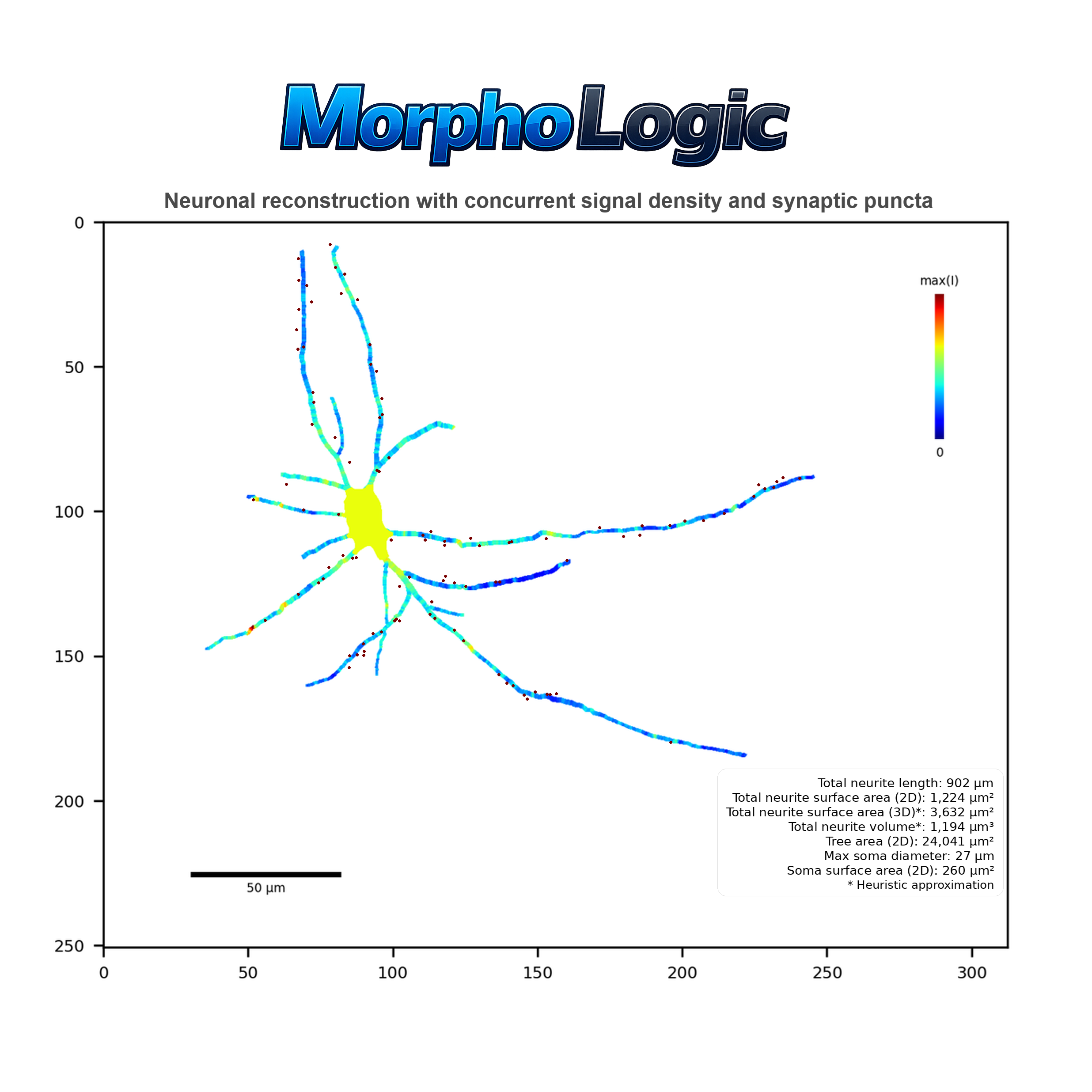
Signal
An overlay where neurites and soma are colored by signal density for each signal channel, normalized within the cell.
Figure 18 - Diagnostic 'Signal' visualization
Notes:
- One image per signal channel.
- Normalization: colors represent relative signal density for that specific cell and channel.
- Neurites: each segment is colored by its local signal density.
- Soma: filled with a single color based on somatic signal density.
- Legend: vertical color bar showing the 0-to-max range.
- Optional: axes/title and a scale bar can be shown if enabled.
Puncta
An overlay with puncta markers drawn as small circles, styled by whether each punctum is assigned to soma or neurites.
Figure 19 - Diagnostic 'Puncta' visualization
Notes:
- Base image: same neurites + soma overlay as 'reconstruction'.
- Puncta sit on top of the reconstruction so they remain visible.
- Puncta style: filled circles with a thin outline ring for contrast.
- Somatic puncta: soma-colored fill with neurite-colored outline.
- Neurite puncta: neurite-colored fill with soma-colored outline.
- Optional: axes/title and a scale bar can be shown if enabled.
Mapping
A summary of morphology-aware mapping curves for the cell: puncta and signal density.
Figure 20 - Diagnostic 'Mapping' visualization
Notes:
- Only distance from soma is visualized as independent variable
- One panel for puncta and one panel for each signal channel analyzed.
- Distance from soma range is trimmed to the largest radius that contains non-zero values.
Sholl
A 2×2 summary of Sholl curves for the cell: intersections, segment lengths, branch points, and terminal points versus radius.
Figure 21 - Diagnostic 'Sholl' visualization
Notes:
- Four panels: intersections, segment lengths, branch points, terminal points (all plotted vs. radius).
- Radius range is trimmed to the largest radius that contains non-zero values.
- Panels include compact summaries such as AUC, critical point, correlation, slope, and total.
Interpret and use aggregated per-dataset tables
15m
Find the aggregated outputs and understand the folder layout
After a run with aggregation enabled, MorphoLogic writes all per-dataset CSV outputs under an “Aggregated” folder inside your dataset parent directory (see Step 8). Step 6 explains that your dataset is organized as a tree of independent-variable folders. During aggregation, MorphoLogic uses those folder levels to create grouping columns. Those groupings are what your aggregated tables summarize. In other words: your folder naming and nesting defines the independent variables; the aggregator reads them and then reports results grouped by them.
Figure 22 - The folder structure of aggregated data tables shows an extensive number of data tables. This allows for easy navigation to the statistics-ready data that you need answer your specific research question.
Notes:
- Inside aggregated, you will see two top-level domains: (1) Geometric and (2) Sholl.
- Inside each domain, tables are organized by statistical subject (what we are summarizing). MorphoLogic offers data aggregation per branch, neurite, and cell. A neuronal cell generally consists of multiple neurites, each with branches that span between branch- and terminal points.
- The output structure is designed so you can navigate to “the kind of biology question” you’re asking. What makes MorphoLogic special is that it also offers morphological profiling of signal- and puncta-related variables. On a statistical level, that means that MorphoLogic quantifies these special dependent variables as a function of independent within-subject variables relating to morphology (distance from soma, neurite radius, branch order, electrotonic distance). This is the data that you will find under the 'Binned' folders of within the Cell and Neurite subject of the Geometric domain. In the 'Unbinned' folders, you will find the same data aggregated not within but over the entire statistical subject.
- Inside, MorphoLogic saves two flavors of tables. (1) Element 'el' tables: per-element values after collapsing segments into the chosen subject (neurite, branch, or cell, binned or not), and (2) Statistical summary 'stats' tables: group-level summary statistics computed from the element table (mean, SEM, count, min, max, median, Q1, Q3). Element tables are usually what you want for distributions, dot plots, and statistical modelling, whereas statistical summary tables are usually what you want for quickly plotting group comparisons.
5m
Choose the correct table for your research question
We understand that it can be difficult to make sense of all tables at once. To help you along, we here explain in detail how we aggregate our data:
Geometric domain
Geometric aggregation starts from segment-level measurements.
- What is a segment? Neuronal reconstructions consist of hierarchically organized nodes with a certain position and radius. Between each adjacent node pair exists a segment. When we say segment-level measurements, imagine a table where each row represents one segment with its morphological parameters (radius, distance from soma, electrotonic distance, branch order) and, if enabled, signal density and puncta counts.
- What does “Binned” vs “Unbinned” mean? Unbinned: one value for the whole subject (e.g., one number per cell). Use when you want overall group comparisons without morphology stratification. Binned: multiple values per subject, stratified by within-neuron morphology bins (e.g., neurite radius in .05 µm steps, distance from soma in 10 µm steps, etc.) This is what you use when you want “morphological profiling,” i.e., how a dependent variable changes as a function of: distance from soma, percent distance, electrotonic distance, radius, or branch order.
- How does aggregation work? The first layer goes from segment to element, where reconstructed segments are collapsed into a biological unit. For branch tables, this means one row per branch (unbinned). For neurite tables, this means one row per neurite (unbinned) or one row per neurite within each morphology bin (binned). For cell tables, this means one row per cell (unbinned) or one row per cell within each morphology bin (binned). During this collapse, continuous measures (e.g., radius, signal density) are averaged within the element; for binned neurite/cell outputs, the averaging is length-weighted so longer segments contribute more than tiny fragments. Count-like puncta measures are summed within the element. This is what produces the element table. The second layer goes from element to group statistics. Here, element values are summarized across your experimental groups (defined by your dataset folder levels, e.g., Batch / Timepoint / Cell line). This is what produces the stats table, which reports descriptive summaries you can plot directly: mean, SEM, count (N), min, max, median, Q1, and Q3.
Sholl domain
Sholl aggregation starts from radius-level measurements.
- What is a Sholl “radius”? Sholl analysis samples the reconstruction at a series of concentric radii from the soma (e.g., every 10 µm). When we say radius-level measurements, imagine a table where each row represents one radius value for one cell (or one neurite), with the Sholl dependents at that radius (intersections, segment lengths, branch points, terminal points).
- What does “Binned” vs “Unbinned” mean? Unbinned: one value for the whole subject (e.g., one number per cell or per neurite) that summarizes the entire Sholl curve. Use this when you want standard group comparisons with a single Sholl complexity metric per element. Binned: multiple values per subject, stratified by Sholl radius. Use this when you want to plot and compare full Sholl curves (metric vs radius) across groups.
- How does aggregation work? The first layer goes from radius rows to element, where Sholl measurements are collapsed into a biological unit. For cell tables, this means one row per cell (unbinned; curve compressed into single-number descriptors like AUC/crit/R/slope/total) or one row per cell at each Sholl radius (binned; the full curve retained, keyed by radius). For neurite tables, this means one row per neurite (unbinned; the same curve-descriptor compression) or one row per neurite at each Sholl radius (binned; the full curve retained, keyed by radius). This is what produces the element table. The second layer goes from element to group statistics. Here, element values are summarized across your experimental groups (defined by your dataset folder levels). The stats tables report descriptive summaries you can plot directly: mean, SEM, count (N), min, max, median, Q1, and Q3.
10m
Protocol references
- Schindelin J, Arganda-Carreras I, Frise E, et al. Fiji: an open-source platform for biological-image analysis. Nature Methods. 2012;9(7):676–682. doi:10.1038/nmeth.2019.
- Schneider CA, Rasband WS, Eliceiri KW. NIH Image to ImageJ: 25 years of image analysis. Nature Methods. 2012;9(7):671–675. doi:10.1038/nmeth.2089.
- Arshadi C, Günther U, Eddison M, Harrington KIS, Ferreira TA. SNT: a unifying toolbox for quantification of neuronal anatomy. Nature Methods. 2021;18(4):374–377. doi:10.1038/s41592-021-01105-7.
- Hunter JD. Matplotlib: A 2D graphics environment. Computing in Science & Engineering. 2007;9(3):90–95. doi:10.1109/MCSE.2007.55.
- Harris CR, Millman KJ, van der Walt SJ, et al. Array programming with NumPy. Nature. 2020;585:357–362. doi:10.1038/s41586-020-2649-2.
- Virtanen P, Gommers R, Oliphant TE, et al. SciPy 1.0: fundamental algorithms for scientific computing in Python. Nature Methods. 2020;17(3):261–272. doi:10.1038/s41592-019-0686-2.
- McKinney W. Data Structures for Statistical Computing in Python. Proceedings of the 9th Python in Science Conference (SciPy 2010). 2010. doi:10.25080/Majora-92bf1922-00a.
- da Costa-Luis CO. tqdm: A Fast, Extensible Progress Meter for Python and CLI. Journal of Open Source Software. 2019;4(37):1277. doi:10.21105/joss.01277.
- The pandas development team. pandas-dev/pandas: Pandas (v2.3.3) [Software]. Zenodo; 2025. doi:10.5281/zenodo.17229934.
- The Matplotlib Development Team. Matplotlib: Visualization with Python (v3.10.8) [Software]. Zenodo; 2025. doi:10.5281/zenodo.17595503.
- Gommers R, Virtanen P, Haberland M, Burovski E, Reddy T, Weckesser W, et al. SciPy (v1.17.0) [Software]. Zenodo; 2026. doi:10.5281/zenodo.18209846.
- Gillies S, van der Wel C, Van den Bossche J, Taves MW, Arnott J, Ward BC, et al. Shapely (v2.1.2) [Software]. Zenodo; 2025. doi:10.5281/zenodo.17193310.
- da Costa-Luis C, Larroque SK, Altendorf K, Mary H, Richardsheridan, Korobov M, et al. tqdm (v4.67.1) [Software]. Zenodo; 2024. doi:10.5281/zenodo.14231923.
- Gohlke C. tifffile (v2024.8.30) [Software]. Zenodo (concept DOI). doi:10.5281/zenodo.6795860.
- Gohlke C. roifile (v2024.9.15) [Software]. Zenodo (concept DOI). doi:10.5281/zenodo.13765488.
- Rasterio contributors. rasterio (>=1.3) [Software]. Available from: PyPI / GitHub project pages.
- Affine contributors. affine (>=2.4) [Software]. Available from: PyPI / GitHub project pages.
Acknowledgements
We thank Dr. Moritz Negwer for thoughtful guidance on the structure of the publication, and Dr. Dirk Schubert and Lucas van Grootveld for productive discussions on morphometry conventions. We are also grateful to colleagues in the Nael Nadif Kasri lab for beta testing MorphoLogic on their datasets and for identifying issues that improved robustness and usability. We additionally thank Prof. Paul Tiesinga for generously providing access to cluster compute resources and storage that supported development. We acknowledge GitHub for code hosting and version control, and protocols.io for providing this excellent platform for sharing and maintaining versioned methods. This work was supported by the Netherlands Organization for Scientific Research, NWO NWA.1518.22.136 SCANNER, to N.N.K. in support of M.L.S.