Jul 09, 2025
Modeling the developmental potential of Dirofilaria spp.
- Yury Prilepsky1,2,
- Sergey Konyaev1,3
- 1Institute of Systematics and Ecology of Animals of the Siberian Branch of the RAS, Novosibirsk, Russian Federation;
- 2e-mail: [email protected];
- 3e-mail: [email protected]
- Yury Prilepsky: conception, design; adaptation of R script;
- Sergey Konyaev: validation of the protocol;


Protocol Citation: Yury Prilepsky, Sergey Konyaev 2025. Modeling the developmental potential of Dirofilaria spp.. protocols.io https://dx.doi.org/10.17504/protocols.io.e6nvwqro7vmk/v1
License: This is an open access protocol distributed under the terms of the Creative Commons Attribution License, which permits unrestricted use, distribution, and reproduction in any medium, provided the original author and source are credited
Protocol status: Working
We use this protocol and it's working
Created: May 30, 2025
Last Modified: July 09, 2025
Protocol Integer ID: 219186
Keywords: Ecology, EIP, Temperature, Larvae, Dirofilaria, developmental potential of dirofilaria spp, temperature requirements for the extrinsic incubation period, dirofilaria spp, extrinsic incubation period, dirofilaria, temperature condition, temperature requirement
Funders Acknowledgements:
Federal Basic Scientific Research Program
Grant ID: FWGS-2021-0001
Abstract
We aimed to analyze temperature requirements for the extrinsic incubation period (EIP) completion to identify where and when Dirofilaria spp. transmission is possible. A map was created illustrating areas where, based on temperature conditions from 2006 to 2016, the EIP of Dirofilaria spp. could be completed: year-round, for more or less than six months, or never.
Guidelines
Dirofilaria spp. are filarial nematodes transmitted by intermediate hosts—mosquitoes. The parasite primarily infects domestic dogs but can also infect other animals, including cats, and may affect humans.
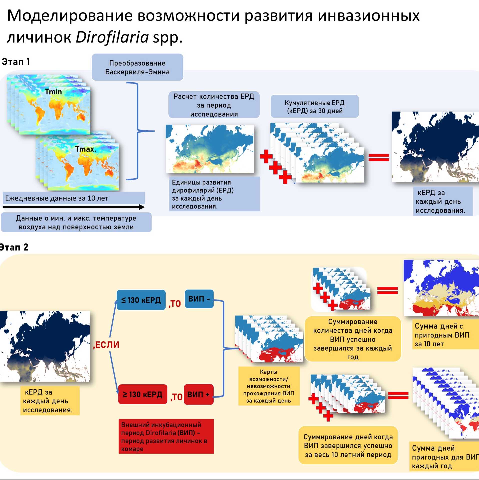
The life cycle of Dirofilaria spp. involves two phases: infection of the definitive host with L3 larvae via mosquito bites, development into adult worms in the definitive host’s tissues, and release of microfilariae into the bloodstream. The microfilariae are then transmitted back to a mosquito, which serves as the intermediate host. Inside the mosquito, Dirofilaria larvae complete the extrinsic incubation period (EIP), undergoing two developmental stages (L1–L3) before becoming infective to a new host. Larval development within the mosquito requires a specific amount of heat (measured in Dirofilaria development units, DDUs), which depends on ambient temperature. The rate of larval development from L1 to L3 is positively correlated with ambient temperature and has a minimum developmental threshold of 14°C [1; 2]. Assuming a mosquito ingests microfilariae on the first day of its adult life, completing the EIP (i.e., accumulating the required minimum of 130 DDUs) within its 30-day lifespan would require a mean daily temperature of 19.3°C (equivalent to a mean daily DDU accumulation of 4.3). At higher mean daily temperatures, the process would complete in fewer than 30 days. Studies indicate that the likelihood of Dirofilaria transmission varies by geographic location and season. We aimed to analyze temperature requirements for EIP completion to identify where and when Dirofilaria spp. transmission is possible across Russia. A map was created illustrating areas where, based on temperature conditions from 2006 to 2016, the EIP of Dirofilaria spp. could be completed: year-round, for more or less than six months, or never.
R script was developed by a research team studying Dirofilaria development suitability in Australia [3]. We express our deep gratitude for the brevity, efficiency, and open-access availability of their code. To assess climatic suitability in all world, the script was modified. In its current form, the script processes daily raster data from CHELSA and can calculate temperature suitability for Dirofilaria EIP completion worldwide.
Materials
To develop maps assessing temperature suitability for Dirofilaria spp. development in intermediate hosts, we analyzed geographic (raster) data. The study utilized gridded datasets where information was stored as uniformly sized pixels, comprising 250,560 cells with a resolution of 1800 arcseconds (equivalent to 30 arcminutes or 0.5°).
Each cell contained daily temperature values for a 10-year period, including:
- Maximum daily near-surface air temperature (tasmax, °K)
- Minimum daily near-surface air temperature (tasmin, °K)
These data covered global spatial extent.
Computational Methods
All calculations were performed using:
- R programming language (v4.4.2)
- Key R packages: raster , terra , sf , sp , maps, ncdf4 , tidyr
Before start
Before proceeding with the analysis, it is necessary to download raster temperature data from the CHELSA project website at the required spatial resolution.
To streamline the workflow, we recommend:
- Creating a dedicated working directory for each project.
- Setting this directory as the working directory in R (e.g., using setwd() function or RStudio projects).
This approach ensures organized file management and reproducibility.
Load required R packages
Software
R programming language
NAME
The R Foundation
DEVELOPER
REPOSITORY
SOURCE LINK
Load required packages for R
library(ncdf4); library(ggplot2); library(rasterVis);
library(maps); library(tidync); library(devtools)
library(terra); library(viridis); library(raster)
library(dplyr); library(readr); library(purrr); library(stringr)
library(tibble); library(magick); library(aws.s3); library(rasterVis)
library(devtools); library(spatialkernel);
library(rmapshaper); library(cmsaf)
Stage 1: Daily DDU raster calculation
Rasters generated in Step 1 display the absolute number of degree-days above 14°C (the minimum temperature threshold required for Dirofilaria spp. larval development in intermediate hosts) for each calendar day.
To create these maps, we utilized open-access climate data from CHELSA [4], which provides daily maximum (tasmax) and minimum (tasmin) temperature data in WGS84 geographic coordinates (EPSG:4326). A total of 8,036 daily raster files were processed, covering the period from 1 January 2006 to 31 December 2016 (10 calendar years).
Dataset
CHELSA-W5E5 v1.0: W5E5 v1.0 downscaled with CHELSA v2.0
NAME
Daily Development Units (DDUs) were calculated using the Baskerville-Emin method [5], which models diurnal temperature variation as a sine curve between Tmin and Tmax. The DDU calculation for each raster cell was performed as follows:
# Creating daily DDU rasters
# Generate date sequence from 01-01-2006 to 31-12-2016 by month
dseq <- seq(from = as.Date("01-01-2006", format =
"%d-%m-%Y"),
to = as.Date("31-12-2016", format = "%d-%m-%Y"), by =
"month")
# Set output filenames for:
# 1. DDU rasters
ddu.pname <- paste("DDU/ddu", format(dseq, format =
"%Y%m%d"), ".nc", sep = "")
# 2. Minimum temperature inputs
ddu.pname_min <- paste("temp/Tempmin/chelsa-w5e5_obsclim_tasmin_1800arcsec_lat-90.0to90.0lon-180.0to180.0_daily_",
format(dseq, format = "%Y%m"), ".nc", sep =
"")
# 3. Maximum temperature inputs
ddu.pname_max <-
paste("temp/Tempmax/chelsa-w5e5_obsclim_tasmax_1800arcsec_lat-90.0to90.0lon-180.0to180.0_daily_",
format(dseq, format = "%Y%m"), ".nc", sep =
"")
#=====================================================================
# Concatenate monthly netCDF files into single files
cmsaf.cat(var = "tasmin", infiles = ddu.pname_min, outfile =
"Tempmin")
cmsaf.cat(var = "tasmax", infiles = ddu.pname_max, outfile =
"Tempmax")
fn <- "Tempmin.nc" # Consolidated minimum temp file
fx <- "Tempmax.nc" # Consolidated maximum temp file
# Create RasterBrick for daily minimum temperature
for(i in 1:length(dseq)){
trasbrick <- brick(fn)
tmin.r <- subset(trasbrick, i:i) # Extract ith layer
# Repeat for maximum temperature
trasbrick <- brick(fx)
tmax.r <- subset(trasbrick, i:i)
# Calculate daily mean temperature (Kelvin)
Tavg <- (tmax.r + tmin.r)/2
# Development threshold parameters
base <- 289 # Base temperature in Kelvin (=14°C)
W <- (tmax.r - tmin.r)/2 # Half daily temperature range
# Calculate angular parameter
Q <- (base - Tavg) / W
# Constrain Q values between -1 and 1
Q[Q < -1] <- -1
Q[Q > 1] <- 1
A <- asin(Q) # Angular transformation
# Daily DDU calculation (thermal development units)
tddu.r <- ((W * cos(A)) - ((base - Tavg) * ((pi / 2) - A))) / pi
# Write DDU raster to GeoTIFF
writeRaster(tddu.r, filename = ddu.pname[i],
format = "GTiff", overwrite = TRUE)
# Progress counter
cat(i, "\n")
flush.console()
}
Daily raster outputs were produced, with each pixel value quantifying accumulated DDUs. Zero-value pixels denoted areas where temperatures remained below the 14°C minimum required for larval development
Map illustrating by color the DDU value as of Febrary 1, 2006
Stage 2: 30-Day cumulative DDU (cDDU) Maps
Subsequently, daily cumulative Dirofilaria development unit (cDDU) maps were generated, representing the total number of Dirofilaria development units (DDU) accumulated over the preceding 30-day period (corresponding to the maximum mosquito lifespan) for each study day from 1 February 2006 to 31 December 2016:
### Daily DDU maps are combined into a raster stack to create cDDU maps
dseq <- seq(from = as.Date("01-01-2006", format =
"%d-%m-%Y"),
to = as.Date("31-12-2016", format = "%d-%m-%Y"), by =
"day")
# Set raster filenames:
ddu.pname <- paste("DDU/ddu", format(dseq, format =
"%Y%m%d"), ".tif", sep = "")
cddu.pname <- paste("ddumaps/cddu", format(dseq, format =
"%Y%m%d"), ".tif", sep = "")
obname <- data.frame(idx = 1:length(ddu.pname), ddu = ddu.pname, cddu =
cddu.pname)
nday <- 30 # 30-day accumulation window
it <- 0
it <- it + 1
dcut <- cut(32:length(dseq), breaks = 10) # Split processing into 10
chunks
dcut.n <- match(dcut, levels(dcut))
ord <- which(dcut.n == it)
ord <- (32:length(dseq))[ord]
for (i in 32:length(dseq)) {
# For each day, select DDU rasters from the previous 30 days:
idx.start <- i - (nday - 1)
idx.stop <- i
idx <- idx.start:idx.stop
tddu.fname <- as.character(obname[idx, 2])
rasters <- 0 # Initialize raster collection
for (j in 1:length(tddu.fname)) {
traster <- rast(tddu.fname[j]) # Read each daily DDU raster
rasters <- c(rasters, traster)
}
rasters <- rasters[-1] # Remove initialization value
tcddu.r <- rast(rasters) # Create raster stack
# Sum all values in the Raster stack (30-day cumulative DDU)
tcddu.r <- app(tcddu.r, fun = sum)
plot(tcddu.r) # Visual verification
# Save the summed raster (cDDU file) in GTiff format:
writeRaster(tcddu.r, filename = cddu.pname[i], overwrite = TRUE)
cat(i, "\n") # Progress indicator
flush.console()
}
Map illustrating by color the cDDU value as of Febrary 1, 2006
Stage 3: Daily EIP suitability classification
The daily BCDDU (binary cDDU) map indicates which global regions have reached the cDDU threshold (≥130 DDU) required for parasite development completion, and which areas had insufficient accumulation (<130 DDU). This map was generated by classifying each daily cDDU layer using the specified threshold.
### Converting cDDU maps to BCDDU
# <130 = EIP impossible, >=130 = EIP possible
# Set raster filenames:
dseq <- seq(from = as.Date("01-02-2006", format =
"%d-%m-%Y"),
to = as.Date("31-12-2016", format = "%d-%m-%Y"), by =
1)
ddu.pname <- paste("DDU/ddu", format(dseq, format =
"%Y%m%d"), ".tif", sep = "")
cddu.pname <- paste("ddumaps/cddumaps/cddu", format(dseq,
format = "%Y%m%d"), ".tif", sep="")
bcddu.pname <- paste("ddumaps/bcddu", format(dseq, format =
"%Y%m%d"), ".tif", sep = "")
for(i in 1:length(dseq)){
# Load cumulative DDU raster
cddu.r <- rast(cddu.pname[i])
# Apply binary classification (threshold = 130 DDU):
# 1 = suitable, 0 = unsuitable
Rn <- app(cddu.r, fun = function(x) {ifelse(x >= 130, 1, 0)})
# Visual quality check
plot(Rn)
# Save binary CDDU
writeRaster(x = Rn, filename = bcddu.pname[i], overwrite = TRUE)
# Progress counter
cat(i, "\n"); flush.console()
}
A dichotomous map showing possible (in red) and impossible (in blue) passage of the EIP on February 1, 2006.
Stage 4: Annual EIP suitability summaries
The annual cumulative map of suitable EIP zones displays territories where:
- Complete EIP was feasible year-round (365 days or 366 in leap years),
- was feasible for more than six months (183 to 364 days),
- was feasible for less than six months (1 to 182 days),
- or could not occur at all
To construct this map, EIP maps were used, with subsequent summation of suitable days per raster cell. Threshold values were then applied to generate the final annual map of suitability zones.
### Creating annual EIP suitability maps
# Set dates for each study year:
yseq <- seq(from=as.Date("2006-02-01"),
to=as.Date("2016-12-31"), by="years")
yseq.df <- data.frame(1:1, yseq, year=strftime(yseq, "%Y"))
# Create reclassification matrix for suitability categorization
subs.mat <- matrix(data=c(-Inf, 129.999, 0,
129.999, Inf, 1,
NA, NA, NA),
ncol=3, byrow=TRUE)
# Generate annual summary maps
for (j in 1:length(yseq.df[,3])){
## Create date sequence for target year
s <- as.Date(paste("01-02", yseq.df[j,3], sep="-"),
format="%d-%m-%Y")
f <- as.Date(paste("31-12", yseq.df[j,3], sep="-"),
format="%d-%m-%Y")
dseq <- seq(from=s, to=f, by=1)
ddu.pname <- paste("DDU/ddu", format(dseq,
format="%Y%m%d"), ".tif", sep="")
cddu.pname <- paste("ddumaps/cddumaps/cddu", format(dseq,
format="%Y%m%d"), ".tif", sep="")
cddu.r <- rast(cddu.pname[1])
cddu.r <- as(cddu.r, "Raster")
stack.r
<- cddu.r
## Create daily binary suitability maps
for(i in 1:length(dseq)){
cddu.r <- rast(cddu.pname[i])
cddu.r <- as(cddu.r, "Raster")
tbcddu.r <- reclassify(cddu.r, subs.mat, include.lowest=TRUE,
right=FALSE)
stack.r <- stack(stack.r, tbcddu.r)
cat(i, "\n"); flush.console()
}
stack.r <- stack.r[[-1]]
tcummul.r <- calc(stack.r, fun=sum)
name <- paste("summarymaps/", yseq.df[j,3],
"_days_at_risk", sep="")
writeRaster(x=tcummul.r, filename=name, overwrite=TRUE,
format="GTiff")
}
# Load first year for classification template
summ.rname <- paste("summarymaps/", yseq.df[1,3],
"_days_at_risk.tif", sep="")
summary.r <- rast(summ.rname)
## Categorize map by days with DDU >130
cuts <- c(-Inf, 0.01, 182.6, 364.9, Inf)
pal <- c("#003CE5", "wheat1",
"goldenrod1", "firebrick2")
Rn <- classify(summary.r, cuts, include.lowest=TRUE, right=FALSE)
plot(Rn)
Rn <- as(Rn, "Raster")
name <- paste("summarymaps/bin", yseq.df[11,1],
"_days_at_risk", sep="")
writeRaster(x=Rn, filename=name, overwrite=TRUE, format="GTiff")
Map illustrating by color the cEIP value as of 2006.
Stage 5: Decadal synthesis (2006-2016)
The decadal suitability map illustrates the spatial distribution of areas where transmission was possible throughout the ten-year study period. The map categorizes territories based on EIP maps: areas with year-round transmission potential (3652 days total), those with transmission occurring more than half of the period (between 1826 and 3651 days), those with transmission less than half the time (1 to 1825 days), and areas without any transmission (0 days).
This composite map was generated by processing all EIP suitability maps from the study period. For each pixel cell, the total number of days meeting transmission criteria was summed. Standard threshold values were then applied to these cumulative totals to produce the final averaged suitability map representing the entire decade.
The methodology maintains consistency with the annual mapping approach while extending the analysis across the full ten-year timeframe. All calculations preserve the original transmission thresholds and spatial resolution used in the daily and annual maps. The resulting visualization provides a comprehensive overview of long-term transmission patterns across the study region.
### Creating 10-year averaged suitability map
dseq <- seq(from = as.Date("01-02-2006", format = "%d-%m-%Y"),
to = as.Date("31-12-2016", format = "%d-%m-%Y"), by = 1)
yseq.df <- plyr::count(data.frame(dseq, year = strftime(dseq, "%Y")), "year")
# Reading daily rasters and preparing raster stack
summ.stackname <- paste(("summarymaps/"), yseq.df[,1], "_days_at_risk.tif", sep="")
stack.r <- stack(summ.stackname)
# Summing all rasters into one
summed.r <- calc(stack.r, sum)
# Categorizing with threshold levels
subs.mat <- matrix(data=c(0, 0.5, 1,
0.5, 1825.5, 2,
1825.5, 3651.5, 3,
3651.5, Inf, 4),
ncol=3, byrow=TRUE)
pal <- c("#003CE5", "cornsilk1", "goldenrod1", "firebrick2")
summed.r <- as(summed.r, "SpatRaster")
Pn <- classify(summed.r, subs.mat, include.lowest=TRUE, right=FALSE)
plot(Pn, col = pal)
writeRaster(x = Pn, filename = "summarymaps/20062016decadesummary.tif", overwrite = TRUE)
Map showing the average EIPs over a ten-year period divided into 4 categories according to the possibility of passing the period: all year (red), half year (orange), less than half year (green) and impossible (blue).
Results
We generated:
- 4,018 daily DDU rasters
- 3,987 cDDU rasters (30-day cumulative)
- 3,987 binary EIP suitability maps
- 10 annual summary maps
- 1 decadal synthesis map
All outputs are available in GeoTIFF format at 0.5° resolution.
Protocol references
1. Christensen, B. M. & Hollander, A. L. Effect of temperature on vector-parasite relationships of Aedes trivittatus and Dirofilaria immitis. Proc Helminthol Soc Wash 45, 115–119 (1978).
2. Fortin, J. F. & Slocombe, J. O. D. Temperature requirements for the development of Dirofilaria immitis in Aedes triseriatus and Ae. vexans. Mosquito News 41, 625–633 (1981).
3. Atkinson, P. J., Stevenson, M., O’Handley, R., Nielsen, T. & Caraguel, C. G. B. Temperature-bounded development of Dirofilaria immitis larvae restricts the geographical distribution and seasonality of its transmission: case study and decision support system for canine heartworm management in Australia. International Journal for Parasitology 54, 311–319 (2024).
4. Karger, D. N., Lange, S., Hari, C., Reyer, C. P. O. & Zimmermann, N. E. CHELSA-W5E5 v1.0: W5E5 v1.0 downscaled with CHELSA v2.0. doi:10.48364/ISIMIP.836809.2.
5. Baskerville, G. L. & Emin, P. Rapid Estimation of Heat Accumulation from Maximum and Minimum Temperatures. Ecology 50, 514–517 (1969).