Jun 19, 2026
Version 2
Mandibular Cross-Sectional Geometry: A systematic image-capture method V.2
- Alejandro Martín Sánchez1,2,3,
- Maria Ana Correia3,
- Patrícia Simão3,
- Ricardo Miguel Godinho3
- 1Universidad Complutense de Madrid;
- 2Universidad Autónoma de Madrid;
- 3Interdisciplinary Center for Archaeology and Evolution of Human Behaviour (ICArHEB), Universidade do Algarve
- Alejandro Martín Sánchez: ORCID: https://orcid.org/0000-0001-6073-8611;
- Maria Ana Correia: ORCID: https://orcid.org/0000-0003-1152-2528;
- Patrícia Simão: ORCID: https://orcid.org/0000-0001-7331-683X
- Ricardo Miguel Godinho: ORCID: https://orcid.org/0000-0003-0107-9577


External link: https://github.com/Alex-Martin1/OrientCSG
Protocol Citation: Alejandro Martín Sánchez, Maria Ana Correia, Patrícia Simão, Ricardo Miguel Godinho 2026. Mandibular Cross-Sectional Geometry: A systematic image-capture method. protocols.io https://dx.doi.org/10.17504/protocols.io.5qpvoez7bl4o/v2Version created by Alejandro Martín Sánchez
Manuscript citation:
To be published
License: This is an open access protocol distributed under the terms of the Creative Commons Attribution License, which permits unrestricted use, distribution, and reproduction in any medium, provided the original author and source are credited
Protocol status: Working
We use this protocol and it's working
Created: June 19, 2026
Last Modified: June 19, 2026
Protocol Integer ID: 319436
Keywords: Cross-Sectional Geometry, Bone cross-section, Human mandible, Archaeology, BoneJ, Amira, Avizo, 3D Slicer, Slicer, open-source, systematic image, systematic approach, capture method
Funders Acknowledgements:
European Union
Grant ID: Erasmus+ programme
Fundação para a Ciência e a Tecnologia
Grant ID: 2022.03020.CEECIND/CP1731/CT0006
Fundação para a Ciência e a Tecnologia
Grant ID: 2023.10993.TENURE.006
Fundação para a Ciência e a Tecnologia
Grant ID: 2022.07737.PTDC
Disclaimer
The European Commission support for the production of this publication does not constitute an endorsement of the contents which reflects the views only of the authors, and the Commission cannot be held responsible for any use which may be made of the information contained therein
Abstract
This protocol provides a detailed description of a systematic approach to obtain mandibular cross-sectional images and extract descriptive variables.
Image Attribution
Cover image: Created by the authors
Guidelines
Typographical emphasis used in the protocol:
- Geometrical concepts and software are in italics, e.g. landmark 1 or Amira (respectively).
- Core concepts (e.g. Alveolar Reference Plane) and reference to images and tables are in bold.
- Software commands, buttons, tools, and actions are indicated using quotation marks (" "), e.g. "Create Object".
- User interface elements are indicated using angle brackets (<>), e.g. <Project View>.
Notes are collapsed by default when their content is recommended but not essential for completing the protocol workflow. Notes that appear expanded by default should be read before proceeding.
This protocol was developed using Amira v2022, 3D Slicer v5.10, Fiji-ImageJ v1.54p, BoneJ, RStudio v2025.05.0+496, and OrientCSG v0.3.4. Different software versions may present slightly different interfaces, but the general workflow should remain the same.
A video overview of the complete workflow is available from the authors upon request.
Materials
- CT-derived virtual mandible datasets, such as DICOM files. Other compatible volumetric formats may also be used when supported by the visualization software, including VOL, ISQ, RAW volumes, TIFF stacks, NRRD files, or MetaImage files (MHD + RAW).
- Amira/Avizo or 3D Slicer for 3D visualization, landmark placement, and automated cross-section orientation using command blocks generated by OrientCSG.
- R version 4.0 or higher. RStudio is recommended for convenience but is not required.
- OrientCSG (at least v0.3.4) installed in R.
- Fiji-ImageJ with the BoneJ plugin installed, for extracting cross-sectional geometry properties from the captured section images.
- A plain-text editor, such as Windows Notepad.
Safety warnings
Although this protocol was designed with reproducibility in mind and can be applied to other skeletal collections, it was developed using a specific sample with particular preservation conditions. As a result, some methodological decisions were shaped by the features and limitations of that sample. Applying the protocol step by step to a different collection may therefore not always be the most appropriate option. Before adopting this workflow, researchers should evaluate the preservation conditions of their own sample, the research questions being addressed, and the software and analytical resources available.
Ethics statement
This protocol is intended for the analysis of human skeletal remains. Before applying the protocol, users must ensure that the study of the material has been authorised by the relevant institutional, curatorial, legal, and/or heritage authorities responsible for the collection under study. Prior approval should be obtained from the appropriate ethics committee or institutional review body, such as an Institutional Review Board (IRB), Human Research Ethics Committee (HREC), Research Ethics Committee (REC), university ethics committee, faculty ethics committee, hospital ethics committee, or other relevant body responsible for research involving human remains.
The use of this protocol does not itself authorise access to human skeletal remains, or their imaging, analysis, or publication. Users are responsible for ensuring that all work complies with applicable ethical standards, legislation, and any additional requirements concerning human remains, including those related to descendant or Indigenous communities.
Before start
Bone cross-sectional morphology responds to mechanical forces by altering the amount and distribution of its bone tissue (Ruff et al., 2006). These changes can be assessed using Cross-Sectional Geometry (CSG), a technique that quantifies the biomechanical properties of bone cross-sections. Studying the biomechanical performance of mandibular cross-sections offers valuable insight into human bone plasticity in response to environmental factors. Specifically, it enables testing whether groups with higher masticatory loads show significant differences in mechanical parameters compared to those with lower masticatory loads (Godinho et al., 2022, 2023). In doing so, this approach evaluates to what extent mandibular morphology is shaped by functional loading, rather than by other neutral factors such as genetic or ontogenetic influences (von Cramon-Taubadel, 2009, 2011, 2014).
Protocol Introduction
Bone remains recovered from archaeological contexts are often fragmented and incomplete, except under exceptional preservation conditions. For this reason, the protocol presented here has been designed from the outset to accommodate both fragmented and complete mandibles. However, to be eligible for analysis, mandibles must retain, at least, one complete dental quadrant, extending from the mesial facet of the first incisor (I1) to the distal facet of the second molar (M2) within the same quadrant; and the alveolar ridges of this quadrant must be well preserved. This requirement is necessary because the protocol relies on generating a reference plane (Toro-Ibacache et al., 2016, 2019) built from alveolar landmarks, which is then used to orient the subsequent data collection planes.
Phase 1: Foundational Framework. Terminology and Core Concepts
In this phase, all the fundamental concepts that serve as the methodological core of the protocol will be defined, namely, the cross-sections, the standardization measurements , the spatial reference points that guide the acquisition of the former (hereafter referred to as landmarks), and the main biomechanical properties that will be obtained later .
Note
All decisions regarding the positioning and orientation of the cross-sections, as well as the selection of measurements for future standardization, were made with the aim of addressing specific research questions in a sample with particular characteristics, determined by our specific case study. The number, location, and orientation of mandibular cross-sections should be determined according to the research objectives and the potential for meaningful comparison with previously published studies. In other research contexts, with different goals or samples that differ in key aspects -especially in terms of preservation-, it may be necessary to partially modify some of the methodological choices presented here, as these directly influence the nature of the results obtained.
To ensure consistency across specimens and to support systematic data acquisition, the first step is to select the appropriate set of anatomical landmarks for each specimen. These landmarks are used to:
- Define the reference plane, referred to as the Alveolar Reference Plane (ARP). This is a key element of the protocol, as it systematizes the orientation of all subsequent cross-sections. The ARP is defined by three specific landmarks: landmark 1, landmark 2 and landmark 1_Line (defined in ). In complete-arch cases, landmark 1_Line can be directly landmarked instead of estimated.
- Guide the acquisition of three biomechanically relevant cross-sections, which intersect specific groups of these landmarks.
- Standardize the collection of linear measurements (later used for size standardization).
Note
The different landmarking workflows described below mainly affect the availability and computation of the linear measurements later used for size assessment or size standardization . In the 9-, 11-, and 12-landmark workflows with an estimated LM1_Line, the logic used to orient the three cross-sections remains unchanged. In complete-arch workflows, however, the orientation logic is still the same, but the geometric source of some orientation vectors changes because LM1_Line is directly landmarked rather than estimated.
Nevertheless, this protocol does not assume that all specimens must be represented by a single fixed landmark configuration. Because archaeological mandibles often differ substantially in preservation, OrientCSG (see below ) supports several landmark sets and preservation modes (Table 1).
Table 1. Mandibular landmark configurations supported by OrientCSG according to preservation status. These standard configurations assume that LM9 can be placed on a real gonion. If LM9 cannot be landmarked and a placeholder is used only to preserve the input structure, set "lm9_valid = FALSE" in "orient_mandible()" (see below). In that case, measurements depending on LM9 are returned as non-computable.
Note
Special preservation cases not directly represented in Table 1
The landmark sets listed in Table 1 cover the standard preservation situations. However, some specimens may not fit these configurations exactly. For example, a specimen may preserve both gonia but lack the mandibular condyle and/or the C-P3 junctions; preserve the mandibular condyle and C-P3 junction but lack both gonia; or lack the gonion, mandibular condyle, and C-P3 junction altogether. In these cases, alternative workflows can be used, but they must be documented clearly:
- If both gonia are preserved but mandibular length cannot be computed, use the 9-landmark workflow to orient the cross-sections, and measure bigonial breadth separately, either directly in the virtual environment or in R using dist3() on the two gonion coordinates.
- If the mandibular condyle and C-P3 junction are preserved but no gonion is available, use the 11-landmark workflow with a placeholder for LM9 and set "lm9_valid = FALSE". This allows OrientCSG to orient the cross-sections and compute mandibular length, while returning measurements that depend on LM9, such as corpus length and bigonial breadth, as non-computable.
- If neither the gonion nor the landmarks required for mandibular length are preserved, use the 9-landmark workflow with a placeholder for LM9 and set "lm9_valid = FALSE". The cross-sections can still be oriented, but corpus length, mandibular length, and bigonial breadth are not computable.
These special cases show that OrientCSG can be adapted to most preservation situations, but the user must ensure that only anatomically valid measurements are retained.
Default 11-landmark protocolFrom 23 to 48 steps
This case applies when one mandibular side is sufficiently preserved to place LM1-LM11 (see below), including one gonion, one mandibular condyle, and one C-P3 junction, but the contralateral gonion is not available as a real anatomical landmark. In this case, the OrientCSG R package estimates the contralateral side geometrically where needed
The default workflow of this protocol uses the 11-landmark configuration listed in Table 2 and shown in Image 1.
Table 2. List of the 11 anatomical landmarks of the default protocol and its definitions.
Image 1. Anatomical landmarks used to define the Alveolar Reference Plane (ARP), guide cross-sectional acquisition and subsequent size-standardization.
We collected three cross-sections (Image 2), using the previously defined landmarks to guide their acquisition. The anatomical definitions and biomechanical rationale for each section are presented in Table 3.
Table 3. Anatomical definition and biomechanical rationale for selected cross-sections.
Image 2. Cross-sections intersecting biomechanically relevant regions, all oriented perpendicular to the Alveolar Reference Plane (green line).
Note
Across the 9-, 11-, and 12-landmark workflows described above, the basic orientation logic of the cross-sections is unchanged. In standard incomplete-arch cases, these workflows differ mainly in the linear measurements that are computed later. Only complete-arch cases change how some geometric reference elements are obtained, because LM1_Line is directly landmarked rather than estimated geometrically.
To conclude the foundational framework, we provide a brief description of the main (and most informative) cross-sectional properties used in biomechanical Cross-Sectional Geometry analyses. This explanation is not required to continue with the protocol, so it can be skipped.
Note
- Cortical Area (CA). This variable represents the amount of cortical tissue present in a cross-section, measured in mm². It is proportional to the structure’s ability to resist deformation under pure compression and tension loads.
- Second Moments of Area (I). This variable is proportional to a structure’s resistance to bending in a given plane -when calculated about a specific axis of the section- and to torsion -when calculated about the section’s centroid-. The second moments of area most commonly used in behavioral analyses are the second moment of area about the minimum (Imin) and maximum (Imax) axes of the section, as well as those about the anatomical x-axis (medio-lateral in the mandibular corpus, but antero-posterior in the symphysis) (Ix) and the anatomical superior-inferior axis (Iy). Values are expressed in mm⁴.
- Shape indices (Imin/Imax or Ix/Iy). This variable is calculated by dividing two second moments of area measured along perpendicular axes. Analogous to traditional mandibular “robusticity” indices, it provides information about the distribution of mechanically relevant cortical material for resisting bending forces
Prior to their use in behavioral analyses, these properties may undergo a process of size standardization, as described starting from . Moreover, the interpretation of each of these variables varies depending on the specific mandibular region analyzed (corpus, ramus, or symphysis) and the biomechanical performance model used as a reference.
For a more detailed account of these properties definitions and mechanical implications, see Ruff (2018 and references therein).
*Special attention must be paid to the way Second Moments of Area (I) are labeled, as programs such as BoneJ return Imax and Imin based on the axes described above, whereas most CSG-oriented publications define Imax and Imin based on value (that is, the largest I as Imax, and the smallest as Imin). This distinction is critical because, due to the morphology of bone cross-sections, values calculated about the minimum axis are often higher, while those about the maximum axis are lower. Since virtually all CSG-based studies adopt the value-based nomenclature rather than axis-based, it is easy to misinterpret or mislabel the results if using BoneJ without adjusting for this discrepancy.
Select the software route used to implement the protocol. For this protocol, volumetric datasets -as DICOM, an international standard for storing, transmitting, and managing medical images and related data- can be processed following two software routes:
- Amira/Avizo route. This is the default route, as it was the original implementation and remains the preferred route because of its convenience for visualizing CT data, placing landmarks, and capturing cross-sectional images.
- 3D Slicer route. This alternative route is provided to improve accessibility, reproducibility, and open-science compatibility. 3D Slicer is free, open-source and widely used in biomedical imaging.
Note
The choice between Amira / Avizo and 3D Slicer does not change the anatomical or geometric definition of the cross-sections. It only changes how the volume is loaded, how landmarks are exported or copied, and how the software-specific command blocks generated by OrientCSG are executed.
Importantly, regardless of the route chosen, the same procedure can be applied to other volumetric file formats commonly generated in micro-CT and clinical CT workflows, including VOL, ISQ, RAW volumes, TIFF stacks, NRRD files, and Meta-Image formats (MHD + RAW).
Default Amira Workflow44 steps
This is the default route described first in the protocol. It was the original implementation used by the authors and remains the preferred route in their own workflow because of its convenience for visualizing CT data, placing landmarks, and capturing cross-sectional images.
First, load the image data from which the cross-sections will be extracted. In this route, the data are processed with Amira / Avizo (v.2022), a commercial 3D image analysis and visualization software package. To load the data into Amira, you can follow this tutorial.
Software
Amira / Avizo
NAME
Windows 10 or 11
OS
Thermo Scientific
DEVELOPER
Note
If this is your first time using Amira, we strongly recommend that before proceeding, you review some introductory tutorials to the program that clarify its basic functions, such as Thermo Fisher's User Guide or YouTube Tutorials, or detailed published protocols, such as Park et al., 2022.
Protocol
CREATED BY
Grace Park
Generate a volume rendering or isosurface of the loaded data for 3D visualization. If needed, follow the tutorial provided here.
Note
Activate the "Orthographic Viewing Mode" to prevent objects from being distorted (see Image 4). You are on orthogonal view when the eye icon displays two parallel lines.
Then, place the 11 landmarks. To standardize landmark placement, minimize intra-observer error and increase the accuracy of the missing landmark estimation process; it is highly recommended to consult the landmark positioning procedure shown in the supplementary video , as well as to follow the guidelines provided in Table 2.
These landmarks can be classified into two types: those required to guide the acquisition of the cross-sections, and those necessary for performing the size standardization process.
Note
Coordinate format and system when using external software
The OrientCSG workflow described here is designed to read two coordinate formats: the Amira landmark-coordinate format used in this route, and the 3D Slicer Markups-style coordinate format described in the Slicer route. If landmarks were collected in another software package, the coordinate table must first be converted to one of these two formats before running "orient_mandible()". The converted table should follow the examples shown in this protocol, especially with respect to landmark order and the columns containing the x, y, and z coordinates. You may use a script, large language AI models or other automated tools to reformat coordinates.
A second precaution concerns the coordinate system. OrientCSG accepts both LPS-like and RAS-like coordinate systems. The default is LPS-like, which is the coordinate convention used in this Amira route. This is also the convention in which 3D Slicer Markups coordinates are commonly written or exported by default, including when coordinates are manually copied and pasted from the software (even if the 3D Slicer interface displays the coordinate columns as R, A, and S, the copied or stored values may correspond to LPS). For this reason, no coordinate-system argument is shown in the script below . If the coordinates were obtained from software that stores or exports coordinates in RAS, or if 3D Slicer coordinates were explicitly saved or extracted as RAS world coordinates, use "lm_coord_system = "RAS"" in orient_mandible().
See the 3D Slicer route in for a more detailed explanation of coordinate-system handling.
This step provides a theoretical explanation of how landmark placement defines the Alveolar Reference Plane (ARP). Landmark placement is used not only to record anatomical reference points, but also to define the ARP, which provides the reference plane for orienting the mandibular cross-sections.
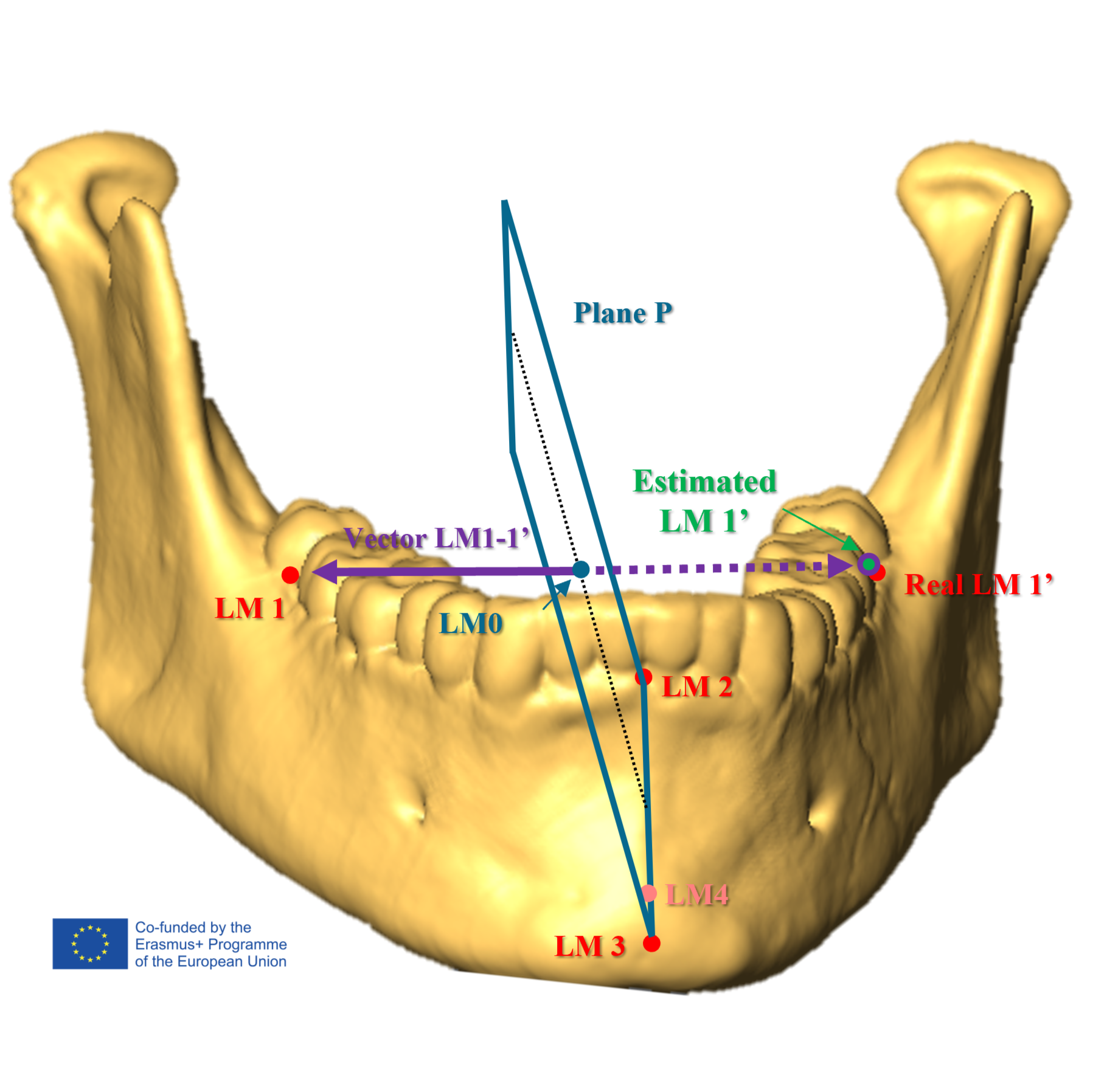
To define a plane in Euclidean space, at least three non-collinear points are necessary. In this workflow, where only one dental quadrant is assumed to be preserved, LM1_Line (or LM1') is not directly landmarked but estimated geometrically. It is computed as the symmetrical reflection of LM1 across a reference plane P, defined by LM2, LM3, and LM4 (Image 3).
Image 3. Graphical representation of landmark 1_Line calculation process.
Note
The calculation of landmark 1_Line involves a series of geometric operations that can be performed manually but are more efficiently handled with the R package OrientCSG, which automates the calculation of this point, generates the geometric elements required for cross-section orientation, and computes the linear measurements used for later size standardization.
Landmarks for ARP definition and cross-section acquisition. Place the landmarks (“LM” from now on) 1 to 8. To achieve this:
- Create a "landmark" object by right-clicking in the <Project View> panel and selecting the option "create object...".
- Search for "Landmarks (Points And Lines)" and select it.
- Rename this dataset (if desired) by right-clicking on the object and selecting "Rename", or by selecting it and pressing "F2".
- Click the <View> tab, located in the upper left corner of the software.
- Search for “Stereoscopic Display” and select "Stereo Test Pattern". This will activate an orthogonal reference grid (Image 4), which will serve as an important visual aid for the accurate placement of landmarks.
- Place the landmarks in their anatomical locations, always in the same order, following the sequence depicted in Table 2 and Images 1, 4 and 5. If you have never placed landmarks in Amira before, consult this tutorial.
Image 4. Amira virtual environment with orthographic view mode and reference grid enabled, illustrating the use of the orthogonal grid to accurately place landmarks 2 and 3.
Note
To ensure accuracy, always adhere strictly to the landmark order outlined in this guide. OrientCSG identifies each landmark based on its position in the sequence. For example, the first point in the dataset will always be interpreted as LM1, regardless of its actual anatomical position. Failing to follow the specified order will therefore result in calculation errors.
Landmarks for size-standardization. Place LMs 9 to 11 following the same procedure and using the same LM dataset as in the previous step. LM10 and LM11 do not necessarily need to be located on the same anatomical side. However, if they are placed on opposite sides, this must be explicitly indicated later when running OrientCSG ( )
Image 5. Superior view of the mandible illustrating the use of the orthogonal grid to accurately place landmarks 5 and 6.
Note
If LM9 cannot be placed on a real anatomical gonion, use a placeholder -a dummy landmark inserted only to preserve the input structure required by "orient_mandible()"- instead. Place this placeholder as close as possible to the expected position of the real gonion. If this is not possible, place it on any preserved inferior point of the mandible. This is important because OrientCSG can use LM9 as an inferior reference to determine the superior-inferior direction of the generated views. For more information, see the penultimate note of .
When using a placeholder for LM9, set "lm9_valid = FALSE". In that case, OrientCSG can still use the available landmarks to orient the cross-sections, but measurements depending on LM9, including corpus length and bigonial breadth, are returned as not computable.
Once the 11 landmarks are correctly positioned, export their coordinates as a .landmarkAscii file. To achieve this:
- Right-click on the "landmark data object" (green module).
- Click on the "folder icon" that appears on the top of the pop-up window (Image 6).
- Select your desired location and save the file with an appropriate name.
- Disable the "Stereo Test Pattern" module by left-clicking on its blue square. The module is considered disabled when the square turns grey.
Image 6. Lateral view of the mandible illustrating landmark placement and the procedure for saving their coordinates.
In this step, the landmark coordinates exported from Amira are processed with the R package OrientCSG in order to:
- Geometrically estimate LM1_Line
- Reconstruct the Alveolar Reference Plane (ARP)
- Compute the orientation elements required for CS1, CS2, and CS3
- Calculate the linear mandibular measurements
- Generate TCL command blocks for Amira, which will be used to orient the ARP, cross-sectional slices, optional "OrthogonalView" object, and camera views.
Note
If this is your first time using R, we strongly recommend that before proceeding, you review some introductory tutorials to the program that clarify its basic functions, such as those offered by RStudio Education. RStudio is recommended for convenience, but it's not required (you can run these commands in any R environment).
Launch RStudio or open the R console (R version 4.0 or higher is recommended). Then run the installation command displayed in the note below (this step is necessary only the first time you use the package).
install.packages("remotes")
remotes::install_github("Alex-Martin1/OrientCSG")
library(OrientCSG)
1. Copy the following command into a new R script.
# 1. Load OrientCSG ====
library(OrientCSG)
# 2. Paste landmark coordinates ====
# Paste below the coordinates exported from Amira.
landmarks_str <- "
PASTE YOUR LANDMARK COORDINATES HERE
"# Coordinates must follow the selected landmark order.
# 3. Run mandibular orientation ====
res <- orient_mandible(
landmarks_str = landmarks_str,
individual_id = "SPECIMEN_ID",
camera_distance_mm = 300,
lm1_side = "RIGHT",
complete_arch = FALSE,
estimate_lm10 = FALSE,
lm9_valid = TRUE
)
# 4. Inspect outputs ====
res
res$summary
res$measurements
# 5. Print Amira TCL blocks ====
cat(get_tcl(res, section = "CS1"))
cat(get_tcl(res, section = "CS2"))
cat(get_tcl(res, section = "CS3"))
# 6. Copy TCL blocks to the clipboard ====
copy_tcl(res, section = "CS1")
copy_tcl(res, section = "CS2")
copy_tcl(res, section = "CS3")
2. Open the .landmarkAscii file exported in with a plain-text editor, such as Windows Notepad, and copy the landmark coordinates.
3. Paste the exported landmark coordinates between the quotation marks in "landmarks_str <-" line. It is essential that the coordinates follow the landmark order defined in Table 2.
4. Replace the SPECIMEN_ID in "individual_id =" argument with the identifier assigned to the specimen under analysis.
For the default 11-landmark workflow, most arguments in "orient_mandible()" can be left as shown in the script. The arguments that may need to be modified depending on specimen preservation and landmark placement are:
- Use "complete_arch = FALSE" when LM1_Line is estimated geometrically from LM1, LM2, LM3, and LM4. Use "complete_arch = TRUE" only in complete-arch workflows, when LM4 is the real LM1_Line.
- Use "lm9_valid = TRUE" when LM9 was placed on a real anatomical gonion. Use "lm9_valid = FALSE" only when LM9 is a placeholder inserted to preserve the input structure. In that case, OrientCSG still uses the available landmarks to orient the cross-sections, but returns measurements depending on LM9, including corpus length and bigonial breadth, as non-computable.
- Use "estimate_lm10 = FALSE" when LM10 and LM11 were placed on the same anatomical side. Use "estimate_lm10 = TRUE" when LM10 and LM11 were placed on opposite anatomical sides. In that case, OrientCSG reflects LM10 across the relevant symmetry plane (see Image 4) and computes mandibular length as LM10_Line-LM11. This option is not applicable to 9-landmark workflows, because LM10 and LM11 are absent.
- camera_distance_mm defines the Amira camera distance when orienting the cross-section view. This affects visualization, not the anatomical calculations.
- lm1_side specifies the anatomical side on which LM1 was placed. Use lm1_side = "RIGHT" when LM1 was placed on the right mandibular corpus, and lm1_side = "LEFT" when LM1 was placed on the left one. This argument is used to orient the generated views consistently for CS1, CS2, and CS3. It does not change the anatomical position of the cross-sections, but it controls the viewing side and the anatomical direction of the generated camera views.
- Some options (as "complete_arch") only need to be changed when using alternative landmark configurations or preservation workflows, as described in the corresponding step-cases.
Note
Geometrically estimated landmarks and measurements should be used with caution. Estimated points such as LM1_Line, LM9_Line, and LM10_Line are derived from symmetry or reflection procedures and therefore introduce additional uncertainty compared with direct measurements between preserved anatomical landmarks. Whether these estimations are acceptable depends on specimen preservation, study aims, and the level of measurement uncertainty considered appropriate by the researcher.
The magnitude of the error introduced by these estimations will be evaluated in a dedicated methodological study currently in preparation.
Once the arguments have been selected according to the preservation and landmarking conditions of the specimen, run the remaining lines of the script until reaching <# 6. Copy TCL blocks to the clipboard>.
The three "copy_tcl()" lines can be run at this stage without causing any problem, but they will need to be run again later from onward, one at a time, when each TCL block is pasted into Amira. Therefore, keep the R session open while continuing with the next steps.
Expected result
After running the script, an object named "res" will be created in R. The script will print two main tables in the R console:
- "res$summary" (Table 4), which contains the geometric components of the computed landmarks, points, and vectors.
- "res$measurements" (Table 5), which contains the linear mandibular measurements that may be used later for size standardization ( ). The status and method columns indicate whether each measurement was directly computed, estimated, or not computable.
If you are working in RStudio, these tables can also be opened with "View()", for example "View(res$summary)". This displays the outputs in a spreadsheet-like viewer within the RStudio environment. Save the coordinates and measurements in your preferred format and environment, for example as .csv files or in an Excel spreadsheet.
Table 4. OrientCSG geometric output for mandibular cross-section orientation.
Table 5. OrientCSG linear mandibular measurements (in mm) for size assessment and standardization
The object "res" also contains two additional outputs that are not printed by default in the script but can be inspected if needed:
- "res$manual_orientation" contains the values needed to check the orientation manually in Amira. This option is available for verification purposes, but it is not recommended as the main workflow because it is slower, more tedious, and more prone to human transcription errors.
- "res$avizo_tcl" contains the TCL command blocks used to orient the ARP, "Slice", "OrthogonalView", and camera views in Amira. These command blocks can be copied by running the final lines of the script, as described below in .
Phase 3: Capture of the cross-sectional images
Return to Amira and create three new objects. These will be configured automatically when the TCL command blocks generated by OrientCSG are run. The required objects are:
- "ARP", a clipping plane used to visualize the Alveolar Reference Plane.
- "OrthogonalView", an optional clipping plane used to verify the orthogonal camera view.
- "Slice", the object that displays the cross-section to be captured.
Note
The object names must be written exactly as shown here. The TCL command blocks generated by OrientCSG identify objects by name. If the names are changed, misspelled, or written with different capitalization, the commands will not configure the objects correctly.
To create the first clipping plane:
- In the <Project View> panel, right-click and choose "Create Object".
- In the search bar, type "Clipping Plane" and select it from the list.
- Rename the new clipping plane object as "ARP".
- In the <Properties> panel of the "ARP" object, open the <Data> tab and select your data source from the dropdown menu (usually a DICOM object).
- The "ARP" object visually represents the Alveolar Reference Plane. Its role is mainly visual and didactic: it allows the user to check the reference plane relative to which the cross-sections are oriented (Images 8 and 9).
Note
ARP manual orientation
Although the "ARP" object is configured automatically through the TCL command block, it can also be oriented manually if needed. However, this is slower, more tedious, and more prone to human transcription errors.
To configure it manually, select the "ARP" object. In the <Properties> panel, expand the <Plane Definition>, and select the "normal & point" option (see Image 11). Then, assign the corresponding components:
- In <Plane Normal>, paste the components of Vec_Penp
- In <Plane Point> paste the coordinates of ARP_Origin
Vec_Penp is the normal vector of the ARP. It is computed from the geometric relationship between Vec_0_2 -direction from LM0 to LM2- and Vec_1_1Line -direction from LM1 to LM1_Line- (see Image 7), where LM0 is the orthogonal projection of LM2 onto the LM1-LM1_Line axis. The sign of this vector is oriented anatomically so that it represents the inferior to superior direction of the generated view.
ARP_Origin is the point used to place the visible plane in Amira. It is calculated as the centroid of the three points that define the ARP (i.e., as mean position of LM1, LM2, and LM1_Line, or as the average of their x, y, and z coordinates). It is not an anatomical landmark and should not be interpreted as one. Its only utility is to display the ARP in the correct position.
The required values can be copied from the "res$summary" or "res$manual_orientation" outputs generated by OrientCSG.
Image 7. Definition of landmark 0 and vector 0-2.
The second object is optional. It is another clipping plane whose function is to verify visually that the camera view generated by the TCL command is orthogonal to the cross-section being captured. To create this object:
- Create another clipping plane, as done in
- Rename the new clipping plane object as "OrthogonalView", respecting capitalization exactly.
- In the <Properties> panel of the "OrthogonalView" object, open the <Data> tab and select your data source from the dropdown menu.
This object is not required for the workflow to run. If "OrthogonalView" does not exist, the corresponding TCL commands will be ignored and the rest of the code will still work.
The final object is the "Slice" object. This is the object that displays the cross-section of interest.
To create it:
- In the <Project View> panel, right-click on the DICOM object and select "Slice". This will create a slice object directly attached to the DICOM data.
- The name of this object must be "Slice", which is usually the default name. If a different name appears, rename it as "Slice". Again, naming is essential for the TCL command to work properly.
- Once created, the "Slice" object will be automatically oriented and positioned when the TCL command block for each cross-section is run.
Note
From this point forward, the term "slice" will always refer to the created object, which appears as an orange-coloured module in Amira (Image 8).
Image 8. Amira objects used by OrientCSG for automated cross-section orientation
After creating the objects required by the TCL command blocks, orient and capture the planned cross-sections. This step outlines the procedural steps that ensure the extracted sections are perfectly perpendicular to the ARP (Image 9).
This workflow is very straightforward. The user only needs to run the corresponding TCL block for each section, visually check the result, and capture the image.
Image 9. Side view of the CS1 capture process, showing the cross-sectional plane intersecting landmarks 5 and 6 and oriented perpendicular to the ARP.
This step explains the procedure for capturing Cross-Section 1 (CS1). To achieve this:
- Ensure that the objects created in are correctly named.
- Return to R or RStudio and run the first line of the section <# 6. Copy TCL blocks to the clipboard>: "copy_tcl(res, section = "CS1")". This will copy the TCL command block required to orient CS1 directly to your clipboard.
- Return to Amira and open the <Consoles> panel. To do this, click the console button located in the lower-right corner of the interface, highlighted with a red square in Image 8.
- Press "Control + V" to paste the copied TCL command block into the <TCL Console> panel, and then press "Enter".
Expected result
After running the TCL command block, Amira should automatically configure the "ARP", "Slice", optional "OrthogonalView", and camera view for CS1 (Images 8 and 10). Check whether:
- The "Slice" object intersects LM5 and LM6 (Image 11)
- The "Slice" object is perpendicular to the "ARP" object.
- The "ARP" object visually represents the Alveolar Reference Plane.
- If the optional "OrthogonalView" object was created, it helps to verify that the generated camera view is orthogonal to the cross-section (Image 10).
If the expected result is not obtained, check the landmark placement and whether the landmarks were pasted into R in the correct order.
Image 10. Cross-sectional slice CS1 aligned to obtain a fully orthogonal view.
Note
Sections appearing upside down
OrientCSG (v0.3.3, not older versions) orients the generated views from anatomical landmark information rather than from the original scanner axes. The right-left direction is defined from the side on which LM1 was placed, specified with lm1_side. The anteroposterior direction is derived from the relationship between LM2 and the LM1-LM1_Line axis. In practical terms, LM2 provides the anterior reference used to orient the mandibular arch relative to the transverse axis. The superior-inferior direction is derived from the ARP normal, whose sign is oriented using the available inferior reference landmarks. OrientCSG first prioritizes a real LM9 when the gonion is preserved ("lm9_valid = TRUE"). If this is not available, LM3 or LM4 may provide the inferior reference depending on the selected landmarking workflow. In complete-arch workflows without a preserved gonion, the placeholder LM9 is used as the inferior reference. For this reason, placeholder LM9 should still be placed on the best available inferior mandibular reference.
Then, if a section appears upside down, mirrored, or viewed from the unexpected side, first check that:
- LM1 was placed on the side indicated by "lm1_side".
- The landmarks were pasted in the correct order.
- "lm_coord_system" matches the coordinates actually pasted into R.
- LM9 was placed on a real gonion, or, when the gonion is not preserved, on a plausible inferior mandibular reference with "lm9_valid = FALSE".
- The generated section intersects the expected anatomical region and is perpendicular to the ARP.
A wrong view orientation does not necessarily mean that the cross-sectional plane was incorrectly defined. If the section passes through the intended region and remains perpendicular to the ARP, but the captured view is still rotated by 180°, the image can be rotated later during post-processing, for example in Fiji-ImageJ.
Note
Set a "safe reference view"
Once the section has been oriented, you can set the standardized view as a safe reference view. To do this, immediately after pasting the TCL command block, and without moving the view, click the <Set Home> button (Image 10). If you have moved the view, run the TCL block again before setting the home view. After this, clicking the <Home> button (Image 10) will return the camera to the standardized CS1 view. This is useful because it allows you to move the camera freely after running the TCL command and then return to the correct view before capturing the image.
Set the view to capture the cross-sectional image. To do this:
- Ensure that the section correctly intersects the region defined by LM5 and LM6 (Image 11).
- Return to the standardized view by clicking the <Home> (see the last note in ) or by running the CS1 TCL command block again.
- Deactivate the visualization of the isosurface, or click the "Clip" icon in the <Properties> panel of the "Slice" object until the CT image is displayed (Image 12, red square).
- Left-click the "Slice" object and go to the <Sampling> section, in the <Properties> panel.
- Check the boxes for "interp. data" and "interp. texture" (Image 10).
- From the drop-down menu, select the “finest” option to improve resolution and tissue definition (Image 10).
- Ensure that the section includes the smallest possible amount of dental tissue (See the collapsed note below for the rationale).
- If the section cuts through a substantial part of a dental root, use the "Translate" tool in the <Properties> panel of the "Slice" object (Image 11) to move the section slightly to a nearby location where less dental tissue is included.
- Once the appropriate section location has been selected, it is recommended to lock the section position by clicking the "Pickable" icon in the <Properties> panel (Image 8).
- If a red point appears on the section, open the <Options> dropdown menu of <Plane Point> and click "Show Points" to deactivate its visualization (Image 10).
Note
The "Translate" tool changes the position of the "Slice" object but does not change its orientation. Small translations can therefore be used to reduce the amount of dental tissue visible in the section while preserving the standardized orientation defined by OrientCSG.
Image 11. Top view of the CS1 capture process showing the cross-sectional plane intersecting landmarks 5 and 6.
Note
Why should dental tissue be excluded from the section? This protocol aims to measure the mechanical properties of mandibular bone, not teeth. Including dental tissue would add material outside the target structure and weaken the modelling assumptions of material homogeneity and bone mechanical responsiveness. For this reason, dental tissue should be minimized whenever possible.
Capture and save the cross-sectional image. To do this:
- In the <Project View> panel, right-click and choose "Create Object".
- In the search bar, type "Scalebars" and select it.
- Adjust the scale properties (left-click in the "Scalebars" object - see Image 12) until it meets your own requirements (Image 14). A recommended scale length is 10 mm.
- Deactivate the display of all other objects except for the "Slice" and the "Scalebars" by clicking on the blue square before the name of the object in the <Project View> panel.
- Adjust the brightness, contrast, and colormap settings until you are satisfied with the visualization. Try to avoid excessive brightness in the enamel and ensure that the cortical bone is clearly visible.
- Zoom in until you are satisfied with the view to be captured.
- Open the <Snapshot> tool (Image 12, red square).
- Choose the .TIF format and select “Grayscale” in the <File options> section (Image 12).
- Save the image using a naming convention that suits you. We recommend saving the image as "individual_CSX", where "individual" is the specimen code and "X" is the section number. Example: For individual “39” and section CS1, 39_CS1.tif.
Image 12. Cross-sectional image capture process.
Skip this step if CS1 was oriented using the TCL command block, as described in . This step is only intended for users who need or prefer to orient the section manually.
Note
Manual orientation of CS1
Although the "Slice" object is configured automatically through the TCL command block, CS1 can also be oriented manually if needed. However, this is not recommended as the main workflow.
To configure it manually:
- Select the "Slice" object. In the <Properties> panel, expand <Plane Definition>, and select the "normal & point" option.
- Then, assign the corresponding components:
- In <Plane Normal>, paste the components of Vec_CS1_Normal.
- In <Plane Point>, paste the coordinates of CS1B.
CS1B corresponds to LM5. Vec_CS1_Normal is the normal vector of CS1. It is computed as the normalized cross product between Vec_CS1 and Vec_Penp. Vec_CS1 is the direction from LM5 to LM6. This means that CS1 contains the LM5-LM6 direction and is perpendicular to the ARP.
The "OrthogonalView" object is optional. It is used only as a visual check that the camera view is orthogonal to the cross-section. To configure it manually:
- Select the "OrthogonalView" object. In the <Properties> panel, expand <Plane Definition>, and select the "normal & point" option.
- Then, assign the corresponding components:
- In <Plane Normal>, paste the components of the CS1 "OrthogonalView" normal reported in the TCL block. These values can be found in the line <catch {"OrthogonalView" normal setCoord 0 x y z}>.
- In <Plane Point>, paste the coordinates of CS1B.
The OrthogonalView normal is derived from Vec_CS1 after projecting it onto the ARP plane. Its purpose is to provide a visual check that the camera view is orthogonal to the cross-section.
The required values can be copied from the "res$summary" or "res$manual_orientation" outputs generated by OrientCSG.
Once the planes have been oriented, manually adjust the view until the "ARP" clipping plane is fully parallel to the upper and lower borders of the screen, and the "OrthogonalView" clipping plane is fully parallel to the lateral borders of the screen. The image should be considered correctly oriented only when both clipping planes appear as straight lines aligned with the screen borders, as shown in Images 8, 9, and 10.
Once this view has been obtained, continue from
This step explains the procedure for capturing Cross-Section 2 (CS2). The process is identical to that of CS1, with the only difference being the two landmarks the slice must intersect. This is because the cross-sectional plane of CS2 shares the same orientation as CS1 along its z-axis (superoinferior), while it differs slightly along its x-axis (mediolateral), as it must intersect landmarks 7 and 8 instead of 5 and 6.
To achieve this:
- Return to R or RStudio and run the second line of the section <# 6. Copy TCL blocks to the clipboard>: "copy_tcl(res, section = "CS2")". This will copy the TCL command block required to orient CS2 directly to your clipboard.
- Return to Amira and open the <Consoles> panel.
- Press "Control + V" to paste the copied TCL command block into the <TCL Console> panel, and then press "Enter".
- Once the standardized view has been obtained, continue from . Save the image using a different name, for example "39_CS2.tif".
Expected result
The resulting view should show:
- The "Slice" object passing through LM7 and LM8 and perpendicular to the "ARP" object.
- The "ARP" object visually representing the Alveolar Reference Plane.
- If the optional "OrthogonalView" object was created, it should help verify that the generated camera view is orthogonal to the cross-section (Image 13).
Note
When the TCL command block for CS2 is executed, the same objects previously used to orient and capture CS1 are reconfigured to capture CS2. If you wish to preserve the CS1 objects, rename them beforehand (for example, by adding a "1" at the end of each object name: "Slice1", "ARP1", and "OrthogonalView1"), and then create three new objects with the names specified in .
Image 13. Cross-sectional slice CS2 aligned to obtain a fully orthogonal view.
Skip this step if CS2 was oriented using the TCL command block, as described in . This step is only intended for users who need or prefer to orient the section manually.
Note
Manual orientation of CS2
To configure it manually:
- Select the "Slice" object. In the <Properties> panel, expand <Plane Definition>
- Select the "normal & point" option. Then, assign the corresponding components:
- In <Plane Normal>, paste the components of Vec_CS2_Normal.
- In <Plane Point>, paste the coordinates of CS2B.
CS2B corresponds to LM7. Vec_CS2_Normal is the normal vector of CS2. It is computed as the normalized cross product between Vec_CS2 and Vec_Penp. Vec_CS2 is the direction from LM7 to LM8. Therefore, CS2 contains the LM7-LM8 direction and is perpendicular to the ARP, following the same logic described for CS1.
To configure "OrthogonalView" manually for CS2:
- Select the "OrthogonalView" object. In the <Properties> panel, expand <Plane Definition>, and select the "normal & point" option.
- Then, assign the corresponding components:
- In <Plane Normal>, paste the components of the CS2 "OrthogonalView" normal reported in the TCL block. These values can be found in the line <catch {"OrthogonalView" normal setCoord 0 x y z}>.
- In <Plane Point>, paste the coordinates of CS2B.
For CS2, the OrthogonalView normal is derived from Vec_CS2 after projecting it onto the ARP plane. Its purpose is the same as in CS1: to provide a visual check that the camera view is orthogonal to the cross-section.
The required values can be copied from the "res$summary" or "res$manual_orientation" outputs generated by OrientCSG.
Once the planes have been oriented, manually adjust the view until the "ARP" clipping plane is fully parallel to the upper and lower borders of the screen, and the "OrthogonalView" clipping plane is fully parallel to the lateral borders of the screen. The image should be considered correctly oriented only when both clipping planes appear as straight lines aligned with the screen borders.
Once this view has been obtained, continue from
This step explains the procedure for capturing Cross-Section 3 (CS3), which provides information related to the mandibular symphysis. Its acquisition differs from CS1 and CS2 because it is not guided by a pair of landmarks located on the mandibular corpus. Instead, CS3 is defined as a "normal & point" plane that passes through LM2 and uses the LM1-LM1_Line direction as its normal vector.
To achieve this:
- Return to R or RStudio and run the third line of the section <# 6. Copy TCL blocks to the clipboard>: "copy_tcl(res, section = "CS3")".
- Return to Amira and open the <Consoles> panel.
- Press "Control + V" to paste the copied TCL command block into the <TCL Console> panel, and then press "Enter".
- The resulting view will be generated from the side specified in the "lm1_side" argument (by default, "RIGHT") in .
- Once the standardized view has been obtained, continue from . Save the image using a different name, for example "39_CS3.tif".
- Check the note below.
Expected result
The resulting view should show:
- The "Slice" object passing through LM2 and perpendicular to the LM1-LM1_Line direction.
- The "ARP" object visually representing the Alveolar Reference Plane.
- If the optional "OrthogonalView" object was created, it should help verify that the generated camera view is orthogonal to the cross-section (Image 14).
- The resulting view will be generated from the side specified in the lm1_side argument
Image 14. Lateral view from the right side of the CS3 capture process, showing the cross-sectional plane intersecting LM2 and oriented according to the LM1–LM1_Line direction.
Note
These steps should be systematically repeated for each specimen in our sample, capturing as many sections as feasible in each instance.
Avoid cross-sections that exhibit orientation impossibility, fragmented bone, absence thereof, or antemortem tooth loss.
It is strongly recommended to organize the output by creating dedicated folders for each individual, naming each folder using the assigned individual label used in your study.
Skip this step if CS3 was oriented using the TCL command block, as described in . This step is only intended for users who need or prefer to orient the section manually.
Note
Manual orientation of CS3
To configure it manually:
- Select the "Slice" object. In the <Properties> panel, expand <Plane Definition>.
- Select the "normal & point" option. Then, assign the corresponding components:
- In <Plane Normal>, paste the components of Vec_1_1Line.
- In <Plane Point>, paste the coordinates of LM2.
Vec_1_1Line is computed as the direction from LM1 to LM1_Line (remember that in the default workflow, LM1_Line is estimated geometrically; but in complete-arch workflows, LM1_Line is directly landmarked as LM4).
To configure "OrthogonalView" manually for CS3:
- Select the "OrthogonalView" object. In the <Properties> panel, expand <Plane Definition>, and select the "normal & point" option.
- Then, assign the corresponding components:
- In <Plane Normal>, paste the components of the CS3 "OrthogonalView" normal reported in the TCL block. These values can be found in the line <catch {"OrthogonalView" normal setCoord 0 x y z}>.
- In <Plane Point>, paste the coordinates of "LM2".
For CS3, the OrthogonalView normal is derived from Vec_0_2 after projecting it onto the ARP plane. Its purpose is the same as in CS1 and CS2.
The required values can be copied from the "res$summary" or "res$manual_orientation" outputs generated by OrientCSG.
Once the planes have been oriented, manually adjust the view until the "ARP" clipping plane is fully parallel to the upper and lower borders of the screen, and the "OrthogonalView" clipping plane is fully parallel to the lateral borders of the screen. The image should be considered correctly oriented only when both clipping planes appear as straight lines aligned with the screen borders.
Once this view has been obtained, continue from
Phase 4. Extraction of cross-sectional properties using BoneJ
Once all cross-sections have been captured and the corresponding images are ready, the next step is to extract their mechanical properties. This analysis is performed using the BoneJ plugin (Domander et al., 2021), which runs within the Fiji-ImageJ platform (Schindelin et al., 2012).
This step describes how to install the software and load the cross-sectional images into it.
- Install Java 8 (required for Fiji to run correctly).
Note
It is recommended to follow the official installation guides at the provided URLs to ensure compatibility and proper setup.
Software
ImageJ (Fiji)
NAME
Windows 10
OS
National Institutes of Health (USA)
DEVELOPER
SOURCE LINK
Once ImageJ is installed and fully functional with the BoneJ plugin, proceed with the following steps to begin mechanical property extraction.
- Open ImageJ.
- Load the desired cross-sectional image by either:
- Pressing "Ctrl + O", locating the file in the appropriate directory, and opening it, or
- Dragging and dropping the image file directly into the ImageJ <toolbar>.
Cross-Sectional Geometry is a technique that focuses exclusively on the mechanical properties of cortical bone. For this reason, before proceeding, remove any visible trace of dental tissue or trabecular bone to avoid distorting the section.
Note
In low-quality CT images where acquisition parameters have not been optimized, distinguishing between cortical and trabecular bone can be challenging. It is strongly recommended not to include any sections in the analysis where the inability to clearly differentiate between cortical and trabecular tissue would result in the inclusion or exclusion of a significant amount of bone.
To remove unwanted tissue from a cross-sectional image in ImageJ:
- Select “Freehand Selection Tool” from the Fiji <toolbar> (see Image 15A).
- Zoom in on the area containing dental structures to be removed.
- Carefully outline the region using the freehand tool. Adjust the threshold value (Image 15B) to assist in tissue selection ( ).
- Once the outline is complete and the shape is closed, press the "Delete" key to remove the selected region (Image 15B).
- To undo an error, press "Ctrl + Z".
Image 15A. Fiji-ImageJ software basics and threshold establishing process.
Image 15B. Cross-sectional image after removal of unwanted tissue.
Note
This step is only necessary if you intend to extract cross-sectional properties oriented with respect to the principal anatomical axes. The decision to acquire these biomechanical parameters will depend on the specific research goals of each project.
In order to do so:
- Go to the <Plugins> tab in the <toolbar>.
- Navigate to "BoneJ" > "Analyze" > "Orientation".
- In the pop-up window, select the appropriate options for your image under “Principal direction” and “Secondary direction” (Image 18).
- Keep the orientation window open. If it is closed, the software will not incorporate the newly defined axes into its calculations.
Note
If the image was captured following the protocol described in previous steps, no manual adjustment should be needed. However, if the orientation needs to be corrected:
- Select the cross-section using the "Rectangle selection mode" (as shown in Image 15)
- Press "Ctrl + X" to cut the selected region.
- Hover the mouse cursor over the orientation crosshair and press "Ctrl + V" to paste it in place (Image 16A).
- Navigate to "Image" > "Transform" > "Rotate..."
- In the pop-up window, enable the "Preview" checkbox while keeping the other settings as default.
- Rotate the image until reaching the desired anatomical orientation (Image 16B).
- Click "OK" to apply the changes.
Image 16. Rotation of the cross-sectional image to its anatomical position.
Note
This step may be skipped if working with high-resolution images, although we still recommend performing it.
This step explains how to convert the cross-sectional images into binary images.
The BoneJ function used to calculate the biomechanical parameters of a section ("Slice Geometry") operates only with binary images (images composed solely of two pixel values - in this case, white and black).
To convert a standard image into a binary one, a threshold must be applied to determine which pixels are converted to black and which to white. Adjusting the limits of this threshold is a key step in extracting the mechanical properties of the sections, as it defines the number and spatial distribution of pixels that the Slice Geometry function will use for its calculations. Therefore, instructions on how to do this are provided from .
Note
If this step is avoided and the function "slice geometry" is applied without previously setting the threshold for transformation, the software will automatically transform the images into a binary format according to its default settings. This is not particularly problematic when working with high-resolution images, but it can significantly compromise the final results if the images are of lower quality, as is often the case with archaeological remains analyzed using medical CT scans.
8-bit images -that is, grayscale images- are the only format that allows binary transformation. If the steps outlined in this guide have been followed, the captured cross-sectional images should already be in 8-bit format (in which case, this step can be skipped). If not, convert them to 8-bit. To do so:
- Hover the mouse over "Image" on the <toolbar> of ImageJ.
- Press "Type".
- Select "8-bit".
To determine the threshold for transforming an image to binary:
- Switch to the "Rectangle Selection Mode" and draw a rectangle around the cross-section (Image 15A, yellow rectangle).
- Press "Ctrl + Shift + C" (or navigate to "Image" > "Adjust" > "Threshold")
- In the pop-up labelled <Threshold> (Image 15A), select “Red” in the right-hand drop-down menu to display thresholded values in red for improved visualization.
From here, you can follow two pathways (it is recommended to try both):
Pathway A. Visual determination of the threshold using thresholding algorithms.
1. In the left drop-down menu, select one of the 16 automatic thresholding algorithms available. To choose the algorithm that best fits your sections, two alternatives can be followed:
- Recommended: Read the note below.
- Alternative: Use “Moments” (Tsai, 1985) or “Minimum” (Prewitt & Mendelsohn, 1966).
2. After selecting the thresholding algorithm, lower the upper threshold value to X + 5, where X is the lower threshold value. In the <Threshold> window, the upper threshold value is positioned below the lower threshold value and is indicated in green in Image 15A. The lower threshold value is positioned above it and is indicated in red in Image 15A.
- To include more tissue, decrease the lower threshold.
- To exclude tissue, increase the lower threshold.
3. Once you are satisfied with the lower threshold value, raise the upper threshold to the maximum (i.e. 255 for a grayscale image).
4. Press “Apply”.
5. Save the lower threshold value used for each specimen’s section, in case it is needed in the future for comparisons or repeating analyses.
Note
To determine the most suitable thresholding method for your study:
- Open 10 cross-sectional images from varied sections and individuals.
- Navigate to "Image" > "Adjust" > "Auto Threshold..."
- In the pop-up window:
- Check “Try all”.
- Press “OK”.
Fiji-ImageJ will display a montage of the 16 available methods applied to your image. Visually compare and select the method that most accurately segments bone tissue for your purposes.
Pathway B. Apply Half-Maximum Height (HMH) thresholding protocol (Coleman & Colbert, 2007; Ulrich et al., 1980). This is -generally- the preferred approach, as it is considered to provide the most reliable estimate of the true boundary between bone and air. However, in low-quality images the method can be difficult to implement and may fail to capture the bone outline accurately. To apply it:
- Close the threshold tab and switch to "Straight Selection Mode".
- Zoom into an area of the contour where the bone–air boundary is clearly visible.
- Draw a line perpendicular to the bone edge that captures a few transitional pixels, including the darkest gray pixel and the brightest bone pixel visible (avoid fully black pixels, as their value of 0 will distort the mean).
- Extract the grayscale or HU profile of this line. To do it, simply press the key "K".
- Record the maximum and minimum gray values. If a fully black pixel was accidentally included, ignore it and take the next minimum value instead.
- Repeat this process by drawing two or three additional lines across different points of the bone–air boundary, and record the maximum and minimum gray values for each one.
- Compute the average of the HMH values obtained across lines.
- The result of the mean value becomes the global threshold for segmenting the full image stack or 3D model.
- To set this value, reopen the <Threshold> window (by pressing Ctrl + Shift + C) and enter the calculated mean in the upper-right field (the lower-threshold box).
- To apply the binarization, press “Apply.”
Expected result
This process, regardless of the pathway chosen, should generate a binary image (Image 18), where:
- White pixels represent bone tissue to be analyzed.
- Black pixels are excluded from calculations.
Establish the scale of the images. To carry this out:
- Switch to the "Straight Selection Mode" (Image 15A) and zoom in on the scale that should be present in the image, as established in .
- Trace the scale line with the mouse, generating a line that best fits the reference length of the image.
- Navigate to the <Analyze> tab on the toolbar and select the "Set Scale" option. This will open a window where the known distance of the object or scale bar (e.g., 10) should be entered in the <Known distance> field, and the corresponding unit of measurement (e.g., mm or millimetres) in the <Unit of length> field.
- Click "OK".
Extract the mechanical properties of our section by applying the Slice Geometry function:
- Go to "Plugins" > "BoneJ" > "Slice Geometry".
- In the pop-up window, select "Mandible" in the <Bone> box.
- Ensure that the "Use orientation" checkbox is selected (if has been completed, it should be active). If not, check it manually (Image 18). If Step 16 was skipped, this checkbox should not be selectable.
- Press "OK".
After processing, a <Results> window will open displaying mechanical variables (some of them described at ) and their values (Image 17A), as well as an annotated image including the axes determined by the maximum and minimum diameters of our section (Image 17B).
Expected result
"Slice Geometry" function outputs.
Image 17A. Table with resulting biomechanical values.
Image 17B. Cross-sectional annotated image.
Save BoneJ outputs:
- Save annotated image using "File" > "Save as" > "Tiff" or "PNG".
- Save the results table as a .csv file in an appropriate location.
Note
Image 18. Extraction of bone cross-sectional properties with Slice Geometry.
Note
Follow this step only if extracting the total surface area of the cross-section (Total Area, TA) and the relative amount of cortical tissue (Percentage Cortical Area, %CA) is required. Otherwise, skip to
To accomplish this:
- Return to the tab containing the binary image (thresholded) of the processed section.
- Select it using the "Rectangle Selection Mode".
- Go to "Process" > "Binary" > "Fill holes". This action creates a filled (solid) version of the section.
- Repeat , which will result in the creation of a new row in our results table. The value recorded in the "CSA" (Cross-Sectional Area) column, which denotes TA in mm², is the only one of interest of this new row.
- Save the resulting value and, if desired, the annotated image from this procedure (although this is not required).
Once all relevant information (annotated images and threshold lower value) has been properly saved, organized, and clearly named:
- Close the cross-sectional image tab and the annotated image tab, taking care not to close the <Results> table, the Fiji-ImageJ <toolbar>, or the <orientation tab>.
- Then, and repeat the full workflow for each additional cross-section to be included in the analysis.
After all sections have been analysed and the .csv file(s) containing all the necessary information have been obtained, compile your results in your preferred platform (e.g., Excel, SPSS or RStudio).
This is the stage where any additional variables which may be beneficial for future analyses can be incorporated, such as %CA (calculated as CA/TA × 100) or the various shape indices ( ).
Note
It is recommended that, when saving the resulting biomechanical values, the column names for Imax and Imin be switched, naming Imax the column previously labeled as Imin, and vice versa, if there is an intention to store both. For an explanation of this adjustment, read the note below on 'Second Moments of Area (I)' in .
Phase 5. Standardization of Cross-Sectional Properties
The standardization process aims to normalize variables by accounting for size-related variation, thereby minimizing the influence of absolute bone size on analytical outcomes. According to Holmes and Ruff (2011), size-standardizing biomechanical values from mandibular cross-sections is only necessary when the groups being compared differ in size. Following their approach, this protocol proposes the collection of five different measurements that:
- Act as proxies for mandibular size, allowing assessment of whether size standardization is required in the specific analytical context
- In case standardization is deemed necessary, can be used to size-standardize the raw biomechanical values.
Note
Before proceeding, it is important to note that alternative methodological approaches exist. These do not consider the need for size standardization based on whether there are significant differences in mandibular size between the groups being compared; instead, they apply standardization as a default step (e.g., Fukase & Suwa, 2008; Antón et al., 2011). The choice of which approach to adopt depends on the judgment of the researcher responsible for conducting the analysis.
The linear measurements, which should have been obtained during , are the following:
- Corpus length. Distance in millimeters between landmarks 3 and 9 (Image 1, ). This measurement is computed only when LM9 is a real anatomical gonion ("lm9_valid = TRUE"). If LM9 was inserted only as a placeholder ("lm9_valid = FALSE"), corpus length is returned as non-computable and must not be used for size assessment or standardization.
- Mandibular length. Similar to that defined by Holmes and Ruff (2011), distance in millimeters between landmarks 10 and 11. In 11- and 12-landmark workflows, this measurement is computed directly when LM10 and LM11 are on the same anatomical side. If they are on opposite sides, set "estimate_lm10 = TRUE" to estimate LM10_Line by reflection and compute mandibular length as LM10_Line-LM11. In 9-landmark workflows, mandibular length is not computable.
- Dental arch breadth: Distance in millimeters between landmarks 1 and 1_Line. In the standard workflow ("complete_arch = FALSE"), LM1_Line is estimated geometrically and dental arch breadth is estimated. In complete-arch workflows ("complete_arch = TRUE"), LM4 is the real A_Line and dental arch breadth is computed directly.
- Dental arch superior length: Distance in millimeters between landmarks 2 and 0 (Image 7). LM0 is the orthogonal projection of LM2 onto the LM1–LM1_Line axis.
- Bigonial breadth: Distance in millimeters between LM9 and the contralateral gonion. In 12-landmark workflows, this measurement is computed directly as LM9-LM12. In 9- and 11-landmark workflows, if "lm9_valid = TRUE", it is estimated as LM9-LM9_Line. If "lm9_valid = FALSE", bigonial breadth is returned as non-computable.
Note
On the Selection of Standardizing Measures
According to Ruff (2000), mechanical stresses (e.g., bending, torsional strength) should be scaled relative to a moment arm – a linear distance from the axis of force application. Ideally, a unique moment arm would be used for each variable and anatomical axis (Dobson & Trinkaus, 2002; Fukase & Suwa, 2008). However, archaeological preservation constraints often limit the availability of precise reference points. Consequently, many studies adopt a reduced number of standardizing measures (e.g., Holmes & Ruff, 2011; May et al., 2018; Sella-Tunis et al., 2018; Toro-Ibacache et al., 2019).
The choice of standardizing measurements must balance methodological rigor with the preservation quality of the skeletal material.
In our case study, these measurements were selected based on the recommendations of other authors as a means to standardize the variables. This does not imply that our approach is the only or the most appropriate one, as other options available in the literature may be more suitable depending on the reader's objectives, possibilities and/or preferences.
Use a statistical test (such as a mean comparison test) to evaluate differences between groups with respect to the previously defined size-related measurements:
- If significant differences are found in any of the mandibular size proxies, full standardization of all biomechanical variables is recommended.
- If the groups under comparison do not differ significantly in mandibular size, the non-adjusted variables can be considered ready for group-comparison analyses.
If needed (see ), apply the following standardization formulas to the second moments of area (I values):
- For mandibular corpus cross-sections (CS1 and CS2):
- Divide Second Moments of Area calculated about the mediolateral (x) and minimum axes (Ix and Imax, respectively) by the (estimated) mandibular length² (Holmes & Ruff, 2011). If LM11 (mandibular condyle) was not acquired (see Note in ), use corpus length² instead (Antón et al., 2011; Daegling & McGraw, 2007; Organ et al., 2006).
- Divide Second Moments of Area calculated about the mediolateral (y) and maximum axes (Iy and Imin, respectively) by the (estimated) bigonial breadth² (Antón et al., 2006).
- For mandibular symphysis cross-section (CS3):
- Divide Second Moments of Area calculated about the antero-posterior (x) and minimum axes (Ix and Imax, respectively) by the (estimated) dental arch breadth² (Daegling, 2001; Dobson & Trinkaus, 2002)
- Divide Second Moments of Area calculated about the mediolateral (y) and maximum axes (Iy and Imin, respectively) by the dental arch superior length² (Dobson & Trinkaus, 2002).
Note
All of these operations can be carried out using the preferred software, whether it be RStudio, Excel, or any other tool of choice. With this, we would have standardized our variables, thus making them ready to be used in various statistical analyses.
Supplementary video available upon request
A support visual guide showing the complete image-capture workflow described in this protocol, from to , is available upon request. This video complements the written instructions and may be useful for visualizing the full sequence of operations in Amira and R.
To request access, contact: [email protected]
Protocol references
Coleman, M. N., & Colbert, M. W. (2007). Technical note: CT thresholding protocols for taking measurements on three‐dimensional models. American Journal of Physical Anthropology, 133(1), 723–725. https://doi.org/10.1002/ajpa.20583
Daegling, D.J. (2001), Biomechanical scaling of the hominoid mandibular symphysis. Journal of Morphology, 250, 12-23. https://doi.org/10.1002/jmor.1055
Daegling, D.J. & McGraw, W.S. (2007). Functional morphology of the mangabey mandibular corpus: Relationship to dental specializations and feeding behavior. American Journal of Physical Anthropology, 134, 50-62. https://doi.org/10.1002/ajpa.20621
Decaup, P.-H., Couture, C., & Garot, E. (2023). Is the distribution of cortical bone in the mandibular corpus and symphysis linked to loading environment in modern humans? A systematic review. Archives of Oral Biology, 152, 105718. https://doi.org/10.1016/j.archoralbio.2023.105718
Dobson, S. D. & Trinkaus, E. (2002). Cross-sectional geometry and morphology of the mandibular symphysis in Middle and Late Pleistocene Homo. Journal of Human Evolution, 43(1),
67–87. https://doi.org/10.1006/jhev.2002.0563
Domander, R., Felder, A. A., & Doube, M. (2021). BoneJ2 - refactoring established research software. Wellcome Open Research, 6, 37. https://doi.org/10.12688/wellcomeopenres.16619.2
Fukase, H. & Suwa, G. (2008). Growth-related changes in prehistoric Jomon and modern Japanese mandibles with emphasis on cortical bone distribution. American Journal of Physical Anthropology, 136(4), 441–454. https://doi.org/10.1002/ajpa.20828
Godinho, R. M., O’Higgins, P., & Gonçalves, C. (2020). Assessing the reliability of virtual reconstruction of mandibles. American Journal of Physical Anthropology, 172(4), 723–734. https://doi.org/10.1002/ajpa.24095
Godinho, R. M., Umbelino, C., Garcia, S., & Gonçalves, C. (2023). Changes in dental wear magnitude in the last ∼8000 years in southwestern Iberia. Archives of Oral Biology, 147, 105626. https://doi.org/10.1016/j.archoralbio.2023.105626
Godinho, R. M., Umbelino, C., & Gonçalves, C. (2022). Mesolithic and Chalcolithic Mandibular Morphology: Using Geometric Morphometrics to Reconstruct Incomplete Specimens and Analyse Morphology. Open Archaeology, 8(1), 536–549. https://doi.org/10.1515/opar-2022-0247
Holmes, M. A., & Ruff, C. B. (2011). Dietary effects on development of the human mandibular corpus. American Journal of Physical Anthropology, 145(4), 615–628. https://doi.org/10.1002/ajpa.21554
Hylander, W. L. (1979). Mandibular function in Galago crassicaudatus and Macaca fascicularis: An in vivo approach to Stress Analysis of the mandible. Journal of Morphology, 159(2), 253–296. https://doi.org/10.1002/jmor.1051590208
Organ, J.M., Ruff, C.B., Teaford, M.F.& Nisbett, R.A. (2006). Do mandibular cross-sectional properties and dental microwear give similar dietary signals?. American Journal of Physical Anthropology, 130, 501-507. https://doi.org/10.1002/ajpa.20377
Park, G., Forknall, N., Heinrich, L., Ludwig, H., Parekh, R., Petruncio, A., Price, J., Ramirez, D., Rymert, Saalfeld, S., Suleiman, A., Vorimo, R., & Weigel, A. (2022). Amira Annotation Protocol V.3. Https://Www.Protocols.Io/View/Amira-Annotation-Protocol-Bp2l61rb5vqe/V1.
Prewitt, J. M. S., & Mendelsohn, M. L. (1966). THE ANALYSIS OF CELL IMAGES*. Annals of the New York Academy of Sciences, 128(3), 1035–1053. https://doi.org/10.1111/j.1749-6632.1965.tb11715.x
Ruff, C. B. (2000). Body size, body shape, and long bone strength in modern humans. Journal of Human Evolution, 38(2), 269–290. https://doi.org/10.1006/jhev.1999.0322
Ruff, C. B. (2018). Biomechanical Analyses of Archaeological Human Skeletons. In M. A. Katzenberg & A. L. Grauer (Eds.), Biological Anthropology of the Human Skeleton. John Wiley & Sons, Inc. https://doi.org/10.1002/9781119151647.ch6
Ruff, C. B., Holt, B., & Trinkaus, E. (2006). Who’s afraid of the big bad Wolff?: “Wolff’s law” and bone functional adaptation. American Journal of Physical Anthropology, 129(4), 484–498. https://doi.org/10.1002/ajpa.20371
Schindelin, J., Arganda-Carreras, I., Frise, E., Kaynig, V., Longair, M., Pietzsch, T., Preibisch, S., Rueden, C., Saalfeld, S., Schmid, B., Tinevez, J.-Y., White, D. J., Hartenstein, V., Eliceiri, K., Tomancak, P., & Cardona, A. (2012). Fiji: an open-source platform for biological-image analysis. Nature Methods, 9(7), 676–682. https://doi.org/10.1038/nmeth.2019
Tsai, W.-H. (1985). Moment-preserving thresholding: A new approach. Computer Vision, Graphics, and Image Processing, 29(3), 377–393. https://doi.org/10.1016/0734-189X(85)90133-1
Ullrich, C. G., Binet, E. F., Sanecki, M. G., & Kieffer, S. A. (1980). Quantitative assessment of the lumbar spinal canal by computed tomography. Radiology, 134(1), 137–143. https://doi.org/10.1148/radiology.134.1.7350593
von Cramon-Taubadel, N. (2009). Revisiting the homoiology hypothesis: the impact of phenotypic plasticity on the reconstruction of human population history from craniometric data. Journal of Human Evolution, 57(2), 179–190. https://doi.org/10.1016/j.jhevol.2009.05.009
von Cramon-Taubadel, N. (2011). Global human mandibular variation reflects differences in agricultural and hunter-gatherer subsistence strategies. Proceedings of the National Academy of Sciences, 108(49), 19546–19551. https://doi.org/10.1073/pnas.1113050108
von Cramon-Taubadel, N. (2014). Evolutionary insights into global patterns of human cranial diversity: population history, climatic and dietary effects. Journal of Anthropological Sciences = Rivista Di Antropologia : JASS, 92, 43–77. https://doi.org/10.4436/jass.91010
Acknowledgements
A Martín-Sánchez is funded by Ministerio de Ciencia, Innovación y Universidades (contract reference FPU24/00394)
MA Correia is funded by Fundação para a Ciência e a Tecnologia (FCT; contract reference 2022.03020.CEECIND; https://doi.org/10.54499/2022.03020.CEECIND/CP1731/CT0006).
P. Simão is funded by a Research Grant within the FCT R&D research project “ParaFunction” (project reference 2022.07737.PTDC; DOI: https://doi.org/10.54499/2022.07737.PTDC).
RM Godinho is funded by Fundação para a Ciência e a Tecnologia (FCT; contract reference 2023.10993.TENURE.006)
This research was also funded by the FCT R&D research project “ParaFunction” (project reference 2022.07737.PTDC; DOI: https://doi.org/10.54499/2022.07737.PTDC)