Feb 24, 2026
Version 1
Littorina saxatilis shell digitization V.1
- David Carmelet-Rescan1
- 1Stazione Zoologica Anto Dohrn, Naples


Protocol Citation: David Carmelet-Rescan 2026. Littorina saxatilis shell digitization. protocols.io https://dx.doi.org/10.17504/protocols.io.8epv5kbd4v1b/v1
License: This is an open access protocol distributed under the terms of the Creative Commons Attribution License, which permits unrestricted use, distribution, and reproduction in any medium, provided the original author and source are credited
Protocol status: Working
We use this protocol and it's working
Created: September 29, 2025
Last Modified: February 24, 2026
Protocol Integer ID: 228429
Keywords: littorina saxatili, morphometric approach, based geometric morphometric, placement andoutline extraction, shellshaper, geometric morphometric, digitization, digitization this protocol detail
Abstract
This protocol details step-by-step procedures landmark placement andoutline extraction, in Littorina saxatilis, ensuring consistency across three morphometric approaches: elliptical Fourier analysis, landmark-based geometric morphometrics, and the growth-based model implemented in ShellShaper.
Photography
Necessary material
- Pink playdough
- Scale (e.g., Graph paper)
- Stereomicroscope with a mounted digital camera
- Label with unique specimen IDs
Snail position
Put the shell on the playdough following these guidelines:
To prepare the shell for imaging, secure it in a petri dish on a bed of soft pink playdough, ensuring the pink background is visible around the entire shell. Position the shell according to the standardized viewing instructions provided below.
Correct Orientation:
- Lateral View: The shell's axis (blue line) must be parallel to the surface when viewed from both the left and right sides.
- Aperture View: When looking directly at the aperture, it should appear flat. The lines along its sides (red and yellow) must be exactly overlapping, indicating no tilt.
Incorrect Orientation:
- Lateral View: The shell's axis (blue line) is not parallel to the surface.
- Aperture View: The aperture does not appear flat; the lines along its sides (red and yellow) are not overlapping, indicating an axial tilt.
Once correctly oriented:
- Frame the Shot: Center the shell, ensuring a generous margin of pink playdough is visible on all sides. Position the specimen label and scale within the frame, ensuring they do not overlap the shell. This setup is critical to minimize parallax effects and to provide a consistent, uniform background for subsequent image analysis.
- Configure Lighting & Focus: Use even, diffuse lighting to illuminate the shell uniformly. Eliminate drop shadows on and around the shell. Ensure the entire shell is in sharp focus.
- Capture the Image: Take a high-resolution, top-view image. Save and rename the image with the sample ID and a picture ID.
Shellshaper digitization
Overview
ShellShaper is a MATLAB software package for extracting growth parameters and generating 3D models from 2D photographs of mollusc shells developed by Larsson et al. (2020) (DOI: 10.1098/rsif.2019.0721). The following protocol is adapted from the official Shellshaper manual (URL: https://orda.shef.ac.uk/s/c7755041a4582c60dd7e).
Software and Environment Setup
Required Software
Ensure the following software is installed and licensed on your system:
- MATLAB: Version R2018b or later.
- Required MATLAB Toolboxes:
- Curve Fitting Toolbox
- Image Processing Toolbox
Shellshaper Package Installation
- Obtain the Shellshaper source code by downloading it from the official repository: Source: https://orda.shef.ac.uk/s/c7755041a4582c60dd7e
- Create a folder named Shellshaper in a convenient location (e.g., within your MATLAB default working directory).
- Extract or save all downloaded MATLAB files (*.m, etc.) into this Shellshaper folder.
- In MATLAB, add the Shellshaper folder and its subfolders to the search path. This can be done by right-clicking the folder in the "Current Folder" browser and selecting Add to Path > Selected Folders and Subfolders.
Setup
- Start MATLAB
- Change directory to the folder where you saved the scripts and open the following file: ShellShaper.m
- Change all paths of folders and files to ones that are correct for your file setup. All folders need to exist before running the program.
- Make sure not to accidentally overwrite already existing files unless you want to. Matlab will do this automatically without asking for permission.
Running the program
Run the program by either pressing F5 or the big green arrow button in the tool strip. Make sure to complete the above setup first, and that the current directory is set to the folder containing the scripts.
1. A new window opens containing an image from the selected image folder.
2. Landmark Placement
- Click on the image to position the first point at the apex. Press enter when done.
- The point "Left" and "Right" a nd "Right2" should correspond to the extreme points of the visible whorls. Press enter when done.
- Position the right and left extreme points of the latest whorls similar to figure 1b. Press enter when done.
- Position the circle to match the curvature of the upper par of the aperture, press enter, then extend the elliptic part to match with the outside lip of the aperture downward and press enter, see figure 1b.
- Finally the "Endcolumella" point correspond to the point of the shell spiral axis reach the botom of the shell, it can be placed behind the aperture lip. The "Endsuture" point correspond to the point where the suture between the last whorle and the rest of the shell end. Press enter when done.
- To get the scale correct, find a known distance using the line L, press enter, and input the value in the dialogue box.
3. There will be a pink shell model on top of the image. A dialogue window will open on top of the image asking if the model is good enough. You have 2 options:
• Yes. This is good, saves images of model and model on original image, go to next one.
• No. This is not good, will let you reposition all the objects to find a better approximation. This will also let you rotate the model to inspect it further. Reposition until happy, when it looks good press yes in the pop-up instead.
When placing landmark points, you may need to adjust their position slightly outside or inside the actual shell outline to overlapping shape accuracy.
4. This will open the next image in the folder, repeat procedure.
Figure 1: Input image (a), interactive positioning of objects (b)-(f), output
images (g)-(h).
Before analyzing their own datasets, all new users should first practice with a training dataset of approximately 100 images. This will help familiarize users with the software and ensure consistent data processing.
Shell Outline Digitization Overview
This method generates a binary (black-and-white) outline of a shell from a single photograph, suitable for morphometric analysis via Fourier transform or other outline-based methods. The protocol leverages subject detection (available in Adobe Photoshop or alternatives like Affinity Photo) to automate extraction.
The goal is to generate black and white outline picture of the shell than can be interpreted by morphometric programs as outline directly.
Software
Photoshop CC
NAME
Adobe
DEVELOPER
Running the program
Open the Image
Launch Adobe Photoshop and open the target image (File > Open).
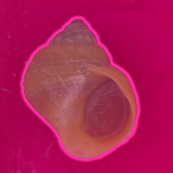
Select the Shell
Use the Object Selection Tool from the toolbar, to click on the shell. Click on the shell structure. A translucent pink overlay will indicate the initial selection.
Refine the Selection
Switch to the Quick Selection Tool to fine-tune the selection. Use the tool to add (+) or remove (-) areas from the selection until the shell's outline is accurately captured. Zoom in as necessary for precision.
Fill the Shell in Black
With the shell selected, navigate to Edit > Fill. In the dialog box, set Contents to Black and Blending Mode to Normal, Opacity to 100%, then Click OK.
Invert the Selection
Navigate to Select > Inverse to select everything except the shell.
Fill the Background in White
With the background selected, navigate to Edit > Fill. In the dialog box, set Contents to White and Blending Mode to Normal, Opacity to 100%, then Click OK.
Export the Final Image
Navigate to File > Export > Save for Web to export the final image with a black shell silhouette on a white background. Save the file using a consistent naming convention.
Repeat this process for each image as needed.
Automating Image Processing in Adobe Photoshop
To improve efficiency, some steps outlined in the previous section (black filling, inversion, white filling, and export) can be automated using the Actions Panel.
Open the Actions Panel
Navigate to the menu bar and select Window > Actions. This will display the panel.
Create a New Action
In the Actions Panel, click the "Create New Action" button (located at the bottom of the panel) and in the dialog box, assign a descriptive name. Click the Record button (circle icon) to begin. All subsequent steps will now be logged.
Record the processing steps.
Manually perform the complete sequence of operations to be automated: filling the subject with black, inverting the selection, filling the background with white, and exporting the image in the desired format.
Stop Recording
Once all steps are complete, click the "Stop Recording" button (square icon) at the bottom of the Actions Panel.
- Apply the Action to Other Images Navigate to File > Automate > Batch. In the Batch dialog box, choose the Action you just created under the Play section.
- Set the Source to Folder, then select Choose.
- Select the folder containing the images you want to process.
- Set the Destination to Folder, then select Choose.
- Select a different folder for Photoshop to output the processed images.
- Check the box beside Override Action “Save As” Commands so that your new files will be saved without prompting.
- In the File Naming section, you can choose how you want your files to be named. Use the pull-down menus to select from predefined options, or type directly into the fields.
Traditional digitization
Traditional digitization involves the manual placement of landmarks and semi-landmarks on shell images using a comb tool. These points are subsequently used for traditional geometric morphometric analysis.
Comb Placement and Alignment
Before placing landmarks, align the digital comb template using vector-editing software (e.g., Adobe Illustrator or Inkscape).
- Position the central yellow line to align with two landmarks: the shell apex (future L1) and the apex of the internal curve between the aperture and the shell body (future L6).
- Align Comb 1 (right) so that its top branch intersects the lower suture of the penultimate whorl (future L4) and its bottom branch contacts the shell's lowest point (future L7).
- Align Comb 2 (left) so that its top branch intersects the upper suture of the penultimate whorl (future L3) and its bottom branch contacts the same internal curve apex as the yellow line (L6).
Correct alignment is shown in Figure 1 and 2.
A downloadable comb template is available at:
Figure 1
Landmark placement
Landmarks can be digitized using the R package Stereomorph (v1.6.7). This package provides a graphical application for consistent point placement.
Load the package and launch the application by running the following code in R.
library(StereoMorph)
digitizeImages(image.file ="path_to_pictures_with_comb_overlay/",shapes.file = "path_to_output/",landmarks.ref = c(1:38))
Follow the on-screen instructions and refer to the official StereoMorph digitizing tutorial for detailed guidance on using the application's tools.
Once the application opens, landmarks must be placed in the precise numerical order shown in Figure 2.
Figure 2.
Description of each landmarks:
L1: apex of the shell
L2: upper suture of the penultimate whorl (right)
L3: upper suture of the penultimate whorl (left)
L4: lower suture of the penultimate whorl (right)
L5: end of the suture
L6: Apex of the inside curve between the aperture and the shell
Line 1: from L1 and L6
L7: Bottom of Comb 1 touches the lowest point of the shell
Line 1: from L1 and L6
Semilandmarks:
L8 - L20: Crossing points between Comb 1 branches and the outer visible margin of the last whorl.
L21 - L33: Crossing points between Comb 1 branches and the aperture inside lip.
L34 - L38: Crossing points between Comb 2 branches and the shell whorl.
Make sure to also place the point defining the scale of the photoraphy and enter the associated distance.
Landmark data are saved in the output folder defined in the orignal codeline.
Data analysis
A comprehensive comparison of data derived from the three digitization techniques described above is presented in the following publication. Please refer to it for detailed analytical methods, statistical procedures, and results.
Link to publication:
Protocol references
Larsson, J., Westram, A. M., Bengmark, S.,
Lundh, T., & Butlin, R. K. (2020). A developmentally descriptive method for
quantifying shape in gastropod shells. Journal of The Royal Society
Interface, 17(163), 20190721. https://doi.org/10.1098/rsif.2019.0721