Dec 18, 2025
Imaging Expanded Mouse Brains on the ExA-SPIM
- Kaelin Wulf1,
- Xiaoyun Jiang1,
- Micah Woodard1,
- Rajvi Javeri1,
- Adam Glaser1
- 1Allen Institute for Neural Dynamics
- Allen Institute for Neural Dynamics


Protocol Citation: Kaelin Wulf, Xiaoyun Jiang, Micah Woodard, Rajvi Javeri, Adam Glaser 2025. Imaging Expanded Mouse Brains on the ExA-SPIM. protocols.io https://dx.doi.org/10.17504/protocols.io.6qpvrwe33lmk/v1
License: This is an open access protocol distributed under the terms of the Creative Commons Attribution License, which permits unrestricted use, distribution, and reproduction in any medium, provided the original author and source are credited
Protocol status: Working
We use this protocol and it's working
Created: July 07, 2025
Last Modified: December 19, 2025
Protocol Integer ID: 221910
Keywords: ExA-SPIM, lightsheet microscope, microscope, expanded tissue, imaging, axial sweeping, mouse, brain, expansion microscopy, imaging expanded mouse brains on the exa, imaging expanded mouse brain, expanded mouse brain, assisted selective plane illumination microscope, brain volumetric image, full neuron reconstruction, microscope, mouse brains for the purpose, sheet microscope, sample holder into the microscope, mouse brain, spim the expansion, imaging, spim software, exa, custom exa, brain, spim
Abstract
The Expansion-Assisted Selective Plane Illumination Microscope (ExA-SPIM) is a custom large-field-of-view axially-swept light-sheet microscope used to image 3x expanded mouse brains for the purpose of full neuron reconstructions. This protocol discusses how to mount the sample holder into the microscope and the steps to acquire a full-brain volumetric image using the custom ExA-SPIM software.
Materials
Supplies:
| Supply | Supplier | Part Number | |
| 1/2" post | Thorlabs | TR2 | |
| Lint free lens cloth | Kimtech | 34120 |
Equipment designed/made in-house (CAD available at https://github.com/AllenNeuralDynamics/exa-spim-hardware):
| Equipment | Part Number | |
| ExA-SPIM Beta microscope | 0329_000-00 | |
| Sample Chamber | 0329_410-00 | |
| Sample holder with glass cuvette | 0329_420-00 |
Buffers/Liquids:
| Liquid | Amount | |
| 0.05X SSC Buffer | 1.5 L | |
| DI water | 2.0 L |
Personal Protective Equipment:
| Suggested PPE | |
| Gloves |
Github repo for Exa-SPIM Imaging GUI: https://github.com/AllenNeuralDynamics/exa-spim-control
Safety warnings
The ExA-SPIM uses class 4 lasers that can reach power levels up to 1 W. Direct exposure to laser light of this power can cause instant eye injury and has the potential to burn skin. The door to the microscope enclosure should never be open when the laser is on, especially if it is turned to higher power levels.
Ethics statement
The protocols.io team notes that research involving animals and humans must be conducted according to internationally-accepted standards and should always have prior approval from an Institutional Ethics Committee or Board.
Before start
This protocol works with tissue that has already been delipidated, immunolabeled, expanded, and mounted (protocol can be viewed here). The sample comes mounted in a sample holder in a container filled with 1.5 liters of 0.05x SSC buffer.
Putting Mounted Sample in Microscope
The sample comes mounted in a covered plastic container. Take note of the ID number, genotype, fluorophore, and buffer listed on the label; the ID will be typed into the software at the end in step 7.5.
Labeled two-quart plastic container covered with aluminum foil containing a mounted expanded mouse brain.
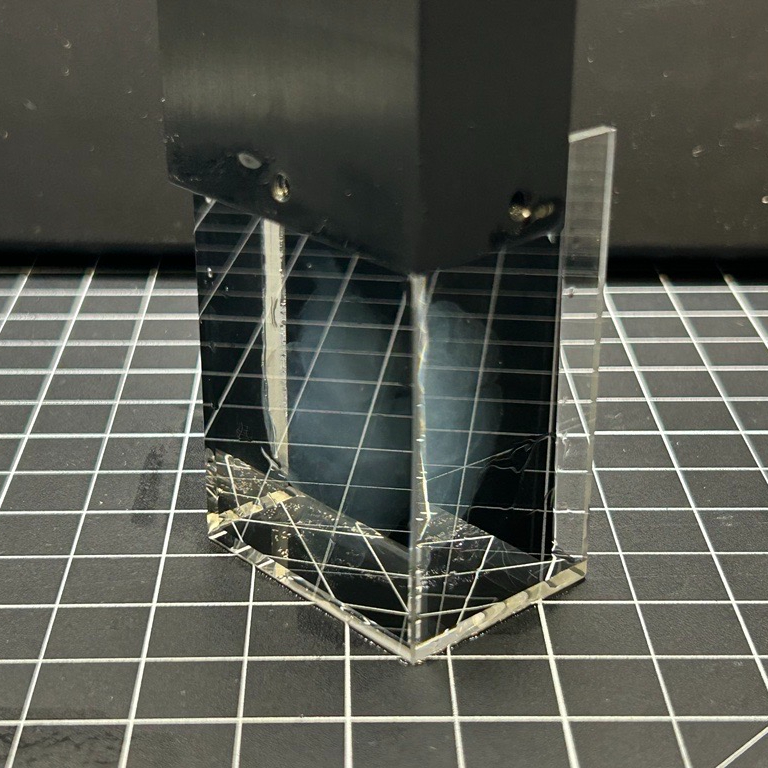
Take the cover off the plastic container and screw a 1/2" post into the center hole at the top of the sample holder. Tighten the rod until snug using a hex key or any other solid rod that can fit to apply more torque.
a) Custom sample holder is shown in 0.05X SSC buffer. b) 1/2" post being tightened into the center hole on the sample holder.
Take the sample chamber from the microscope and rinse it several times with DI water. The DI water can be disposed of in the sink.
Sample chamber being emptied of DI water
Pour out any DI water from the sample chamber and dry with a lint free lens cloth.
Sample chamber being dried with lint free lens cloth
Pour half of the 0.05X SSC buffer from the original plastic container into the sample chamber.
Half of 0.05X SSC buffer being poured from the plastic container into sample chamber.
Quickly transfer the sample holder into the sample chamber to avoid bubbles forming between the hydrogel block and the cuvette walls. Take care to be gentle when placing the sample holder, it will be supported by the glass cuvette resting on the bottom.
Sample holder being transferred to sample chamber.
Then pour the rest of the buffer from the plastic container in to the sample chamber until there is a 1-3 cm gap between the surface of the buffer and the top of the sample chamber. You can lean the sample holder against the wall of the sample chamber in any orientation.
The rest of the 0.05X SSC buffer being poured from the plastic container into the sample chamber.
Place sample chamber onto the chamber mounting plate, being very careful not to bump the illumination subassemblies on the sides. Then lift the sample holder up and place the 1/2" post in the collet and tighten the collet while making sure the rotation of the holder is such that the front of the cuvette is facing towards the detection objective and the sides are parallel with the sides of the chamber. In the image below, the front of the cuvette is facing away from us, so orient the sample holder to match what is seen in the image.
a) Sample chamber with holder being placed onto microscope. b) 1/2" post of sample holder being placed into stage collet and tightened into place.
Software Initialization and Overview
In Visual Studio Code, navigate to the folder that holds the file main.py. Start the software by clicking the arrow in the upper right in the Visual Studio Code window to run the main.py code.
The ExA-SPIM acquisition software uses a GUI built on the Napari viewer. It opens in two windows with all of the necessary widgets visible.
Click the Filter dropdown in the filter wheels widget at the bottom of the lower window and select the appropriate filter for the signal channel. Choose the signal channel based on the fluorophore listed on the sample. If imaging the 561 nm signal channel, select the 620/60BP filter. If imaging the 488 nm signal channel, select the 500LP filter .
Positioning and Defining Edges of the Brain
A different wavelength laser than the wavelength used to excite the neuron-labeling fluorophore can be used to define the bounds of the acquisition. In this case, the 639 nm (red) laser is used in a 561 nm (green) excitable sample. This allows visualization of the brain's shape and structure without bleaching the neuron-labeling fluorophore.
Select the 639 nm laser from the Active Channel dropdown widget in the bottom left corner.
Set the 639 nm laser power to ~35 mW in the box next to the dropdown.
Start the live view by hitting the Live button in the top right area of the window.
Use the joystick to move the brain in X, Y, and Z until tissue is visible in the field-of-view (FOV)
Navigate using the joystick until the olfactory bulbs are in view. They are the most anterior structure in the brain. Depending on the mounting orientation of the brain, they will be at the top or the bottom of the software view. Position them centered in the FOV and scan in and out in Z until the widest section is pictured. Line up the anterior edge of the bulbs with the edge of the FOV, then stop the live view and click the Snapshot button.
In the upper left section, click the plus buttons next to the Rows and Cols until there is a grid with 5 rows and 4 columns. Each tile shown in the grid represents the position of one of the tiles in the acquisition. All the edges of the brain need to fit within the grid so that the whole brain is able to be imaged. A whole 3x expanded mouse brain should be able to fit within this 5x4 tile grid.
Using the joystick, move the FOV until the snapshot of the olfactory bulbs is at the top or bottom edge of the acquisition tiling grid depending on the orientation of the brain; in this case, the snapshot should be moved to the top edge. Make sure there is space visible between the snapshot and the edge of the grid. Then click the Anchor Grid boxes below the first two numbers. This anchors the X and Y movement of the acquisition grid, which enables panning using the joystick without changing the stage acquisition numbers.
Using the joystick, move the FOV down in Y to the center of the grid and then move sideways in X to one of the edges of the grid. This should be where the widest-in-X part of the brain is (cortex).
Resume the live view and scroll in and out in Z until the widest region of the cortex is visible. Line up the edge of the brain with the edge of the FOV. Then pause the live view and hit Snapshot.
Navigate to the other side of the grid and find the opposing widest region of cortex. Then line up the edge of the brain with the edge of the FOV. Pause the live view and hit Snapshot again.
The two most lateral parts of the brain must fit within the grid. If the brain is mounted diagonally or is oversized, adjust the numbers above the Anchor Grid checkboxes and/or adjust the overlap percentage to cover the entire brain with the grid. Any overlap percentage from 5-15% has been shown to be sufficient.
In this case, the brain is oversized. Reducing the overlap percentage from 15% to 6% and adjusting the X-axis anchor numbers allows the grid to cover the entire brain volume.
To check the bottom edge, move the FOV to the bottom of the grid in Y using the joystick, and then center it in X. The hindbrain/spine should be located here.
Resume the live view and move in Z along the spine to find the bottom edge. Once the edge is in view, stop live and click Snapshot.
All of the snapshots to define the XY position of the grid relative to the brain have been set. Adjust the overlap percent and the two anchored numbers until all of the edges of the brain are within the grid
Define Min and Max Z Coordinates
The minimum and maximum Z coordinates must now be defined. Depending on the mounting orientation of the brain, the dorsal/ventral surface could be reversed from what will be described here. In this case, the ventral surface is the Z min and the dorsal surface is the Z max.
The lowest point on the ventral surface could be located either on the spinal cord, another part of the hindbrain, the edges of the cortex, or even in the olfactory bulbs. All of these areas need to be checked to determine where the lowest point is to define the Z min.
Starting in the spine, at the bottom edge of the grid, scroll higher and lower in Z until the visible tissue gets smaller and disappears from the focus. Take note of the the Z position there on a notepad. You will be checking multiple locations for the potential Z minimum, so there is no need to store the value in the software yet.
Move in Y along the center line of the grid to check that the other locations aren't visible at that position. Scroll higher or lower in Z to follow the ventral surface of the brain and keep track of where the FOV is. Once at the ventral cortical area, pan to the left and right in X to check the minimum Z location of both lobes. Whichever brain structure with the lowest position from the list of values you wrote down on a notepad will define the Z min value. Manually type that value in the anchor grid box that corresponds to the Z axis. In this example, the lowest point is in the spinal cord.
In terms of the Z max value, there is a similar process, but it is slightly easier. The highest locations on the dorsal surface are either the cerebellum, or the cortex.
To find the Z max, scroll higher in Z and find where the dorsal edges of those structures disappear from the focus and take note of the Z positions. Choose the maximum position as the Z max
The difference between the Z positions noted in the previous step represents the Z thickness of the sample. However, the number of 1 µm steps that the acquisition takes per tile is quantized in multiples of 2048 µm (2.048mm) so that the resulting images can be easily down-sampled. The scan will automatically round up the Z thickness of the scan to the next multiple of 2.048 mm, but it does so by functionally increasing the Z max value during the acquisition. This would result in extra room on one side of the acquisition but not the other, so instead, you need to even it out and center the sample.
Find out how many multiples of 2.048 mm are necessary to fit the sample. First, take the difference between the Z positions from step 4.2 (in this case 23.5 mm - 3.5 mm = 20 mm), divide that by 2.048 mm (20mm / 2.048 mm = ~9.77), and round up. So that means we need 10 multiples of 2.048 mm to cover the full sample thickness. Center the brain by roughly reducing and increasing the Z min and max numbers until they fill up the full acquisition thickness (in this case we reduce the Z min to 3.3 and increase the Z max to 23.7 which gives us 0.20 mm of buffer space on the Z minimum side and 0.28 mm of buffer space on the Z maximum side.
Now that the acquisition grid space is fully defined, the image quality parameters can be defined.
Setting ETL Offset Parameters
The electrically tunable lens (ETL) is used to sweep the focus of the light-sheet across the FOV. The beam waist must be synchronized with the rolling shutter of the camera or the image will be aberrated axially. The ETL offset determines the position of the waist. Each sample and buffer has slight variations in refractive index, so the ETL offset number needs to be checked and tuned for each sample, and needs to be tuned for both sides of illumination. This step is usually the longest step in the workflow, especially in certain brains that have refractive index inhomogeneities or less than ideal clarity.
To view the labeled neurons, switch the active channel from 639 nm to 561 nm or 488 nm (depending on the labeling). You want to avoid using full laser power while setting up the scan to avoid bleaching. 50-200 mW is recommended for the signal channel laser power while setting up the scan.
When the ETL offset is off from the center, there is effectively a thicker/out-of-focus section of the beam being swept and synchronized with the camera. This leads to a thicker section of the sample being illuminated, meaning out-of-focus sections of neurons will be illuminated in addition to the in-focus ones. When the offset is optimal, the out-of-focus sections go away and there are brighter, smaller sections of neurons. The offset numbers are adjusted in the widget on the right hand side of the GUI as seen below.
This is an example of what the image looks like with a suboptimal ETL offset (4.7 V). Notice how more of the length of the neuron is visible, and the brightness is more diffuse with gradually dimmer edges.
This is an example of what the same image looks like with a more optimal ETL offset (4.9 V). Notice how less of the length of neurons is visible, but the parts that are visible are brighter with sharper edges.
To find the optimal ETL offset, switch back and forth between different offset numbers until gradually centering in on one that looks the best. Write down the offset numbers that look best on a notepad.
The alignment of the ExA-SPIM light-sheet is very sensitive, so it is likely that the optimal offset numbers are slightly different across the full FOV. The difference between optimal numbers from the top to the bottom of the FOV should be within reason (around ±0.03 V), but it is important to notice where in the FOV you are zooming your screen when determining the best offset for that region. The offset should be biased to the center of the FOV because that is usually has the average optimal offset.
Additionally, separate regions of the brain can also have a slightly different refractive index, so the optimal ETL offset may differ between them. For one illumination side, several places along the length of the brain need to be checked, and at different illumination depths. This step can be tedious, but if one or two locations are checked, the optimal offset for the whole brain can be missed. For many brains, the quality of the acquisition is dependent on patience and thoroughness.
For a brain that has labeling everywhere, the main regions to check would be the lateral cortex, the anterior cortex, the dorsal/medial cortex, the olfactory bulbs, medial structures in the brain around the thalamus and hypothalamus, the cerebellum, and the brainstem/spine. For each location, repeat the process for centering in on the optimal offset and take note of that number.
The consistency of the numbers is based on how homogenous the clearing of the brain is. The difference in optimal offset values can range from ±0.01 V to ±0.05 V. Some brains are more consistent than others, so if the optimal offset numbers are very consistent across the first few areas you check (< ±0.02 V), then its likely not necessary to keep checking everywhere.
To find the best ETL offset number for one of the illumination sides, take the different optimal numbers you found for different regions and use the average. For a brain that only has labeling in certain regions, you can bias the offset parameters to that region.
Once the optimal ETL offset number for one side has been found, switch the illumination side with the n_flip_mirror widget and repeat the process for finding the average optimal ETL offset number for the other side.
Setting Focus Parameters
Similar to the ETL offset number, the camera focus needs to be tuned for each sample. However, it is much easier to tune, and much less sensitive. If the focus number is slightly off from the average optimal number, it typically doesn't significantly affect the overall image quality. Generally, the M-stage has a range of ±0.005 mm in which the image stays in focus.
To find the best camera focus, adjust the focus knob on the joystick back and forth and observe how the image gets blurrier and clearer. Center in on the number with the clearest image.
This is an example of what the image looks like with an un-focused camera position.
This is an example of what the image looks like with a focused camera position.
The optimal focus usually doesn't change very much across X and Y in a given Z plane, but different Z planes need to be checked to find the optimal focus throughout the Z depth of the brain. When traveling further from the detection objective, the image usually gets a bit more aberrated, and the optimal focus changes slightly. It is worthwhile to check the areas closest and furthest from the detection path and choose a focus number that makes the furthest areas as clear as possible without making the closest areas notably more out-of-focus.
Once the best focus has been found for one side, write it down and then use the n_flip_mirror widget to switch the illumination sides and find the best focus for the opposite side.
Defining Acquisition
After finding the best ETL offset and focus numbers for the whole brain, the acquisition can be set up. Take note of the anchored stage numbers, the overlap percentage number and the ETL offset numbers and then restart the software to minimize the chance of it crashing during a scan. After booting the software back up, retype the numbers in the appropriate boxes. Redo the grid parameters by creating the 5x4 tile grid with the correct overlap percentage, and re-anchor each of the axis and make sure they have the correct numbers that were noted earlier.
To define the background fluorescence registration channel, click the 'plus' dropdown and select either the 488 nm or 561 nm wavelength (which ever one isn't being used for the signal channel).
The background channel needs to be bright enough, but doesn't need to be high resolution, so we use 8x binning.
This table appears after selecting the wavelength in the previous step. Set up the table as seen below. Change the step size to 8 um, change the binning to 8, change the power to 300 mW if using 488 nm for the background channel. (If using 561 nm, then use 600 mW laser power). Make sure the filter wheel is set to 500LP for 488 nm, or 620/60BP for 561 nm, and change the Round Z box to 256.
To set up the signal channel, add the signal wavelength from the 'plus' dropdown (in this case 561 nm is the signal channel). Make sure the step size is 1 um, and the binning is 1. Set the laser power to 1000 mW. Make sure the filter wheel is set to 620/60BP for 561 nm or 500LP for 488 nm, and make sure the Round Z box is 2048.
Uncheck the "Apply to all" button so that the parameters can be changed per-tile.
Using the camera focus numbers that were noted before, go line by line and change the Camera Position boxes and the N Flip Mirror Position boxes to match which side that tile corresponds to. If using the default stage movement order (row_wise), then the order of N Flip Mirror positions will alternate as seen below.
Repeat this process for the other channel, double checking that the correct focus position corresponds to the correct N Flip Mirror position.
In the Metadata box on the top right, put in the Subject ID according to the label on the sample container
This is the last number to change in the protocol.
Check over all of the numbers that have been put in.
Check that there is at least 10 TB free on the local drive that the files will write to before transferring.
Once everything is fully ready and all of the numbers have been double-checked, click the Start button at the top of the screen. Check in the Visual Studio Code terminal that the acquisition is running normally without any dropped frames. If frames aren't getting getting acquired, or there is an error message, restart the software and start the acquisition again.