Dec 15, 2025
Hypoglossal nucleus analysis from mouse hypoglossal motor neuron stain
- Lucille M Vue1,
- Miranda Cullins1,
- Tiffany J Glass1
- 1Division of Otolaryngology, Department of Surgery, University of Wisconsin-Madison, WI, USA


Protocol Citation: Lucille M Vue, Miranda Cullins, Tiffany J Glass 2025. Hypoglossal nucleus analysis from mouse hypoglossal motor neuron stain. protocols.io https://dx.doi.org/10.17504/protocols.io.q26g71xkqgwz/v1
License: This is an open access protocol distributed under the terms of the Creative Commons Attribution License, which permits unrestricted use, distribution, and reproduction in any medium, provided the original author and source are credited
Protocol status: Working
We use this protocol and it's working
Created: July 08, 2024
Last Modified: December 15, 2025
Protocol Integer ID: 103007
Keywords: analysis, hypoglossal nucleus, mouse, cell count, immunofluorescence, 12N, imageJ, cholinergic neurons, immunofluorescence images of the hypoglossal nucleus motoneuron, mouse hypoglossal motor neuron stain, images available in the hypoglossal nucleus sparc database, hypoglossal nucleus analysis, hypoglossal nucleus motoneuron, cell density hypoglossal nucleus, hypoglossal nucleus sparc database, immunofluorescence image, neuronal nuclei, mouse brainstem, brainstem areas on each section, brainstem area, cell area, antibody
Funders Acknowledgements:
NIH NICHD
Grant ID: R01HD104640-01A1
NIH NIDCD
Grant ID: R01DC019735-01A1
Abstract
This protocol details the analysis process of immunofluorescence images of the hypoglossal nucleus motoneurons in mouse brainstem stained with antibodies targeted against NeuN (Neuronal nuclei) and ChAT (Choline-Acetyltransferase). The analysis can be semi-automatically performed using dedicated ImageJ macro scripts. Data collected from the analysis process contains : cell count, cell area, cell circularity, cell density hypoglossal nucleus and brainstem areas on each section. This analysis was developed to process images available in the Hypoglossal Nucleus SPARC database (DOI : doi.org/10.26275/cnlk-qsai).
Image Attribution
Lucille M Vue, University of Wisconsin-Madison
"Immunofluorescence stain of the mouse hypoglossal nucleus processed and analyzed for neuron count"
Materials
Software :
- Analysis macros (downloadable at
 Macro_HGN_Analysis.ijm Macro_HGN_Conversion_Only.ijm Macro_HGN_Brainstem Trim.ijm Macro_HGN_Trimming.ijm )
Images :
Existing images can be found in the Hypoglossal Nucleus SPARC database (DOI : doi.org/10.26275/cnlk-qsai), or can be generated by following the Hypoglossal Motor Neurons stain of mouse brainstem protocol (DOI : dx.doi.org/10.17504/protocols.io.dm6gpzb6dlzp/v1).
- 10x images of the hypoglossal nucleus stained with anti-NeuN, anti-ChAT and DAPI antibodies, exported as tif raw data (separated layers). These images can be found in the derivative data in sub-mouseID/sam-mouseIDHGN of the SPARC database.
- 4x overview images of the entire slides containing several sections of the mouse brainstem stained with anti-NeuN, anti-ChAT and DAPI antibodies, exported as tif (merged layers). These images can be found in the derivative data in sub-mouseID/sam-mouseIDBS of the SPARC database.
Before start
This protocol is the second entry in a two-part protocol series for hypoglossal neuron count. It requires images obtained from the Hypoglossal Motor Neurons stain of Mouse brainstem available here : dx.doi.org/10.17504/protocols.io.dm6gpzb6dlzp/v1
This analysis uses the ImageJ software and macros that can be both downloaded in the Materials section of this protocol.
Preparations
For this analysis, you will need two sets of images :
- 1 set of 4x overviews of the full slides where all sections taken are imaged. These can be exported as normal tif. If using images from the hypoglossal nucleus SPARC database (DOI : doi.org/10.26275/cnlk-qsai), they can be found in the derivative data in sub-mouseID/sam-mouseIDBS.
- 1 set of 10x images focused on the hypoglossal nucleus for sections which contain it. The number of sections can range from 15 to 25 sections, depending on age. These should be exported as raw data tifs, with no burnt in info in CellSense. If using images from the hypoglossal nucleus SPARC database (DOI : doi.org/10.26275/cnlk-qsai), they can be found in the derivative data in sub-mouseID/sam-mouseIDHGN.
You will also need to create two folders in advance for saving purposes :
- sam-mouseIDHGN-converted will contain the 10x images after being converted from Red-Blue-Cyan to RGB for the analysis to work properly.
- sam-mouseIDHGN-analysis will contain all the files necessary for the analysis as well as the result files.
Example of how the folders should look like.
Finally, you will need ImageJ/Fiji as well as several macros that can be downloaded in the Materials tab.
Brainstem measurement
It is necessary to outline the brainstem area in each section where the hypoglossal nucleus is imaged to relate the size of the hypoglossal nucleus to the brainstem size. This is done on 4x overviews of each entire slide. Identify and count the sections in which the hypoglossal nucleus is present (ChAT+/NeuN+ neurons, appearing respectively in cyan and red). This number should always coincide with the number of 10x photos in the raw image folder.
Load a new macro in ImageJ : Macro_HGN_Brainstem_Trim.ijm and run it. This can be achieved by dragging the file from the the file explorer to ImageJ, then clicking "run".
Select the folder in which the 4x slide overviews are located, then complete the next field with the number of sections in which the hypoglossal nucleus is present. All the overviews should open at once.
Identify the first section in which the hypoglossal nucleus is present (which should coincide with the first 10x image in the raw folder), and use the polygon tool to follow the edges of the brainstem. Do not include the cerebellum. Once the selection is complete, click "ok" in the popup. Do the same with the next section until the brainstems are measured in all sections of interest.
Example of how the selection should look like just before hitting "ok".
Warning ! If you click on "cancel", you will have to close all windows manually and re-run the macro. Moreover, It is important to not click "ok" without being done with the current section selection, and do not re-measure a brainstem that has already been measured. If you do, the section counter might shift and you might not be able to do the measurement on all sections of interest. If you need to append a previously validated selection, select it in the ROI manager, move the selection points to the correct position then click "Update" in the ROI manager.
Once all the brainstems from sections of interest have been measured (the last measured brainstem should coincide with the last 10x image in the raw folder), a window will automatically open to select the saving directory of the brainstem measurements. Select the analysis folder and save it. Once it is done, Fiji will automatically close all the windows.
Hypoglossal nucleus analysis
Pseudo-color conversion
Before analysis of the 10x images, they will need to be converted from Red Blue Cyan to Red Green Blue. This is necessary so that the ChAT signal (cyan) does not split between the green and blue channels of the image when separating the red, green and blue channels of the image.
Select Macro_HGN_Conversion_Only.ijm and drag it to ImageJ. This will open the macro. Click on “Run” at the bottom left of the window.
A popup opens and inquires for input and output directories, as well as file suffix. Browse
the Input directory to select your sam-mouseIDHGN folder, and browse the output directory to select sam-mouseIDHGN-converted. Make sure “.tif” is the File suffix.
Example of the input and output directories filled in the conversion popup.
The images are going to be flashing one by one as they are converted and saved to the output folder. This folder should be looking like this and the images should be in Red Blue Green. Check all the images after conversion to make sure that no image is missing or corrupted. If an image is missing or corrupted, delete all converted images and proceed to a new conversion. If the conversion fails once more, troubleshoot the problem : if the problem is happening to the same image, try reexporting the image.
Example of the contents of the converted folder and how the images look after conversion.
Hypoglossal nucleus trimming
Now that the images have been converted, it is necessary to outline the hypoglossal nucleus in each image so that neurons outside the area of interest are not accounted for. This outline will also allow for a calculation of the area of the hypoglossal nucleus in each section. Drag Macro_HGN_Trimming.ijm to ImageJ and click “Run”. Then select the folder containing the converted images (sam-mouseIDHGN-converted).
Using the polygon selection, encircle the entire hypoglossal nucleus (both left and right nuclei). You should include the area that seems highlighted in green, and not include the dorsal motor nucleus of the vagus (10N) containing ChAT+/NeuN- cells. After closing the selection, click “OK”. Do the same for all the images. When noticing a cell that seems to be ChAT+/NeuN+ outside of the hypoglossal nucleus area, write it down with the animal ID to count the total “perihypoglossal” cells, corresponding to ChAT+/NeuN+ cells locatged lateral to the hypoglossal nucleus.
Examples of hypoglossal nucleus trimming.
After going through the entire stack, a saving popup will appear. Select the analysis folder. The trimmed images will be saved as a tif stack named mouseID age whole HGN.tif
Warning ! If you click on "cancel", you will have to close all windows manually and re-run the macro. Moreover, It is important to not click "ok" without being done with the current section selection, and make sure you do not try to re-measure on a slide or miss one. If you do, the section counter might shift and you might not be able to do the measurement on all slides. Clicking ok automatically puts you on the slide corresponding to the section counter. If you need to append a previously validated selection, select it in the ROI manager, move the selection points to the correct position then click "Update" in the ROI manager. Finally, if a section has been imaged but does not contain any hypoglossal neuron, do not click "ok" as it will fail the macro. Instead, make a small selection not containing any neuron.
Automatic analysis
Now that the hypoglossal nucleus has been trimmed, the analysis and cell count can be performed.
To analyze the whole HGN, drag Macro_HGN_Analysis.ijm to ImageJ and click “Run”. Then select the file mouseID age whole HGN.tif in the analysis folder.
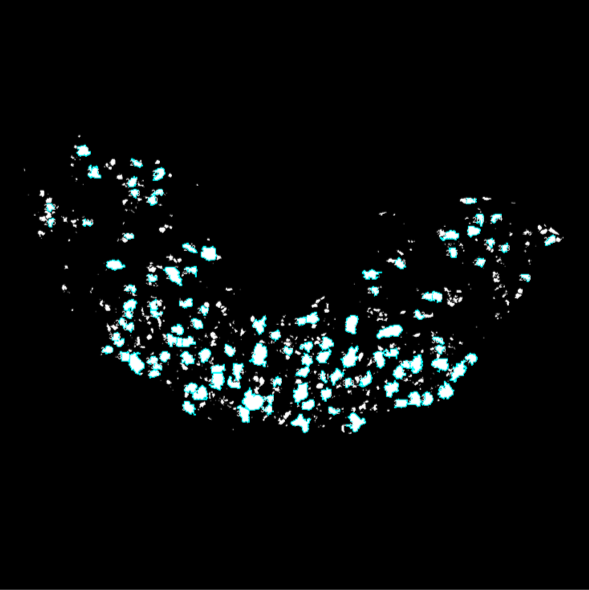
The analysis is performed completely autonomously and will provide binary images of each section in which cells that are both Neun+ and ChAT+ are counted and highlighted in light blue. When you click “OK” to saving the results, the results and their summary will be created in the folder you’re working in, as well as a txt document including all the thresholds automatically picked by the macro and the resulting binary images.
This is an example of the images after being processed and analyzed. The parts in white are areas that are both NeuN+/ChAT+, and the areas circled in cyan are the ones counted as cells in the analysis.
Validation and analyzed variables
Validation
Comparison with a manual analysis.
| Manual Count | Automated Count | |
| 2266 | 2300 | |
| 2163 | 2206 | |
| 1969 | 2017 | |
| 1803 | 1852 |
Comparison of the manual and automated cell counts for a few hypoglossal nuclei from different genotypes and sexes. The automated count is slightly higher than the manual count as it can count some artifacts as cells. However, a Pearson correlation test shows a strong correlation between the two data sets [R2=0.9998 , p=0.0001].
Comparison between different experimentators.
| Experimentator 1 | Experimentator 2 | |
| 2228 | 2291 | |
| 2379 | 2506 | |
| 2136 | 2155 | |
| 2181 | 2311 |
Comparison of the automated cell counts made by two experimentators for a few hypoglossal nuclei from different genotypes. Some differences can be observed in cases where the borders of the hypoglossal nucleus are not clear. If the analysis is to be performed by several experimentators, ensure that they are all properly trained and have agreed on what should or should not be included in the hypoglossal nucleus. A Pearson correlation test shows a good correlation between the two data sets [R2=0.9130 , p=0.0445].
Explanation of the variables studied
Cell density : This is the cell count divided by the sum of the hypoglossal nucleus area in each section, expressed in #/mm2.
The section from the Euploid 20mo female on the left presents a lower cell density (318 cells/mm2) than on that of the Euploid p35 female on the right (411 cells/mm2).
Perihypoglossal cells : This is the proportion of cells lateral to the hypoglossal nucleus on the total cell count in the hypoglossal nucleus. This is not calculated by the analysis macro but needs to be calculated manually from the number of perihypoglossal cells counted during the trimming step, expressed in %.
The section from the Euploid 20mo female on the left presents no misplaced cells compared to that of the Euploid p25 female on the right where 3 misplaced cells are indicated by white arrows.
Cell area : This is the area measurement of each cell that is analyzed, expressed in μm2.
The section from the Euploid 20mo female on the left presents a higher average cell area (564 μm2) than that of the Euploid p36 female on the right (406 μm2). The areas values of a few cells are indicated in black.
Circularity : This is a measurement of how circular the cells are, calculated by ImageJ and going from 0 to 1, 1 being a perfect circle.
The section from the Euploid 20mo female on the left presents lower circularity (0.473) compared to that of the Euploid p35 female on the right (0.581). The circularity values of a few cells are indicated in black.
Area ratio : This is a ratio between the area of the hypoglossal nucleus on the area of the brainstem.
The section from the Ts65Dn 20mo male on the left presents lower area ratio (0.028) compared to that of the Ts65Dn p35 male on the right (0.037). The hypoglossal nucleus is circled in green and the brainstem is circled in yellow, and the area measurements are indicated in the same colors.
Protocol references
Study of neuron morphology and count (cell area, cell circularity, cell count) using ImageJ :
Das, Soumen, and Narendrakumar Ramanan. “Region-Specific Heterogeneity in Neuronal Nuclear Morphology in Young, Aged and in Alzheimer’s Disease Mouse Brains.” Frontiers in Cell and Developmental Biology, vol. 11, Feb. 2023. Frontiers, https://doi.org/10.3389/fcell.2023.1032504.
Fernández-Arjona, María del Mar, et al. “Microglia Morphological Categorization in a Rat Model of Neuroinflammation by Hierarchical Cluster and Principal Components Analysis.” Frontiers in Cellular Neuroscience, vol. 11, Aug. 2017, p. 235. PubMed Central, https://doi.org/10.3389/fncel.2017.00235.
Study of cell density in the hypoglossal nucleus in Sudden Infant death Syndrome :
John R. O'Kusky, Margaret G. Norman, Sudden Infant Death Syndrome: Postnatal Changes in the Numerical Density and Total Number of Neurons in the Hypoglossal Nucleus, Journal of Neuropathology & Experimental Neurology, Volume 51, Issue 6, November 1992, Pages 577–584, https://doi.org/10.1097/00005072-199211000-00002
Neurons located outside of the hypoglossal nucleus (perihypoglossal cells) innervate geniohyoid muscle in rats :
Uemura-Sumi, Masanori, et al. “The Distribution of Hypoglossal Motoneurons in the Dog, Rabbit and Rat.” Anatomy and Embryology, vol. 177, no. 5, Mar. 1988, pp. 389–94. Springer Link, https://doi.org/10.1007/BF00304735.