Dec 23, 2023
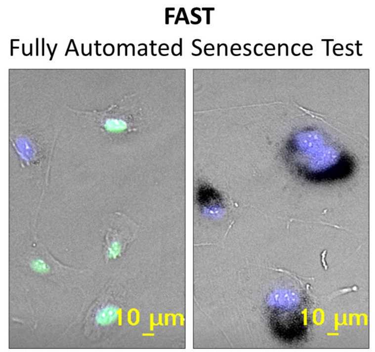
Fully Automated Senescence Test (FAST)
- Francesco Neri1,2,
- Selma N. Takajjart1,
- Chad A. Lerner1,
- Pierre-Yves Desprez1,3,
- Birgit Schilling1,2,
- Judith Campisi1,2,
- Akos A. Gerencser1,4
- 1Buck Institute for Research on Aging;
- 2USC Leonard Davis School of Gerontology;
- 3California Pacific Medical Center;
- 4Image Analyst Software
- Gerencser Lab


Protocol Citation: Francesco Neri, Selma N. Takajjart, Chad A. Lerner, Pierre-Yves Desprez, Birgit Schilling, Judith Campisi, Akos A. Gerencser 2023. Fully Automated Senescence Test (FAST). protocols.io https://dx.doi.org/10.17504/protocols.io.kxygx3ypwg8j/v1
License: This is an open access protocol distributed under the terms of the Creative Commons Attribution License, which permits unrestricted use, distribution, and reproduction in any medium, provided the original author and source are credited
Protocol status: Working
We use this protocol and it's working
Created: August 29, 2023
Last Modified: December 23, 2023
Protocol Integer ID: 87056
Keywords: cell assessment of senescence, cellular senescence, automated senescence test, friendly quantification of senescence burden, positive senescence marker staining, senescence test, quantifies senescence burden, senescence inducer, quantification of senescent cell, cell assessment, senescence burden, senescence, lack of senescence, adopted senescence, senescent cell, markers for each cell, aging field, galactosidase activity, cultured cell, aging, major driver of aging, cell level, quantifying colorimetric sa, single cell level, cell
Abstract
Cellular senescence is a major driver of aging and age-related diseases. Quantification of senescent cells remains challenging due to the lack of senescence-specific markers and generalist, unbiased methodology. Here, we describe the Fully-Automated Senescence Test (FAST), an image-based method for the high-throughput, single-cell assessment of senescence in cultured cells. FAST quantifies three of the most widely adopted senescence-associated markers for each cell imaged: senescence-associated β-galactosidase activity (SA-β-Gal) using X-Gal, proliferation arrest via lack of 5-ethynyl-2’-deoxyuridine (EdU) incorporation, and enlarged morphology via increased nuclear area. The presented workflow entails microplate image acquisition, image processing, data analysis, and graphing. Standardization was achieved by i) quantifying colorimetric SA-β-Gal via optical density; ii) implementing staining background controls; iii) automating image acquisition, image processing, and data analysis. We show that FAST accurately quantifies senescence burden and is agnostic to cell type and microscope setup. Moreover, it effectively mitigates false-positive senescence marker staining, a common issue arising from culturing conditions. Using FAST, we compared X-Gal with fluorescent C12FDG live-cell SA-β-Gal staining on the single-cell level. We observed only a modest correlation between the two, indicating that those stains are not trivially interchangeable. Finally, we provide proof of concept that our method is suitable for screening compounds that exacerbate or mitigate senescence burden (i.e. senescence inducers and senolytics, respectively). This method will be broadly useful to the aging field by enabling rapid, unbiased, and user-friendly quantification of senescence burden in culture, as well as facilitating large-scale experiments that were previously impractical.
Before start
This protocol is for quantifying the senescence-associated markers SA-B-Gal, proliferation arrest (i.e. lack of EdU incorporation), and morphology alteration (i.e. increased nuclear area) of adherent cells cultured in 96-well microplates.
Note
- Ensure to seed cells in a 96W plate suitable for cell culture and immunofluorescence imaging (e.g. Corning, cat# 3904; coverglass-bottomed plates, e.g. Greiner SensoPlate, Cellvis plates)
- Do not seed cells in the wells at the edge of the 96W plate (rows A and H, columns 1 and 12), but fille such wells with PBS. Medium in wells not surrounded (in all directions) by other wells tends to evaporate more quickly, and excessive medium evaporation could affect cells growth and viability.
- For each condition, assign some wells for background staining (no EdU, no X-gal)
Example of plate layout for Senescent and Control cells, culture either at full serum (FS) or in serum-starved conditions (SS):
Protocol Overview
This protocol is for measuring senescence-associated biomarkers by using the FAST workflow.
FAST paper: INSERT LINK
Note that this protocol does NOT include senescence induction methods. To induce senescence in your cell culture model using established methods, some of the most common protocols are available here
The protocol will take roughly 2 days, but multiple pause points are available once the cells are fixed and the SA-B-Gal staining is completed (Day 2).
Example schedule (time indicated refers to a single 96-well microplate):
- Day 0: EdU feeding (10-20 min)
- Day 1: Fixation and overnight SA-B-Gal staining (45-60 min)
- Day 2: EdU detection, image acquisition, image analysis, data analysis (7-8 h)
Reagents
| A | B | C | |
| Item | Company | Catalog | |
| DMSO | ThermoFisher Scientific | BP231-100 | |
| Click-iT EdU Alexa Fluor 488 HCS Assay | ThermoFisher Scientific | C10351 | |
| Senescence Detection Kit, SA-B-Gal kit | BioVision (Abcam) | K320-250 (ab65351) | |
| X-Gal | Life Technologies | 15520-018 | |
| Dulbecco's PBS with Ca2+ & Mg2+ (DPBS) | ThermoFisher Scientific | 14040117 | |
| PBS | ThermoFisher Scientific | 10010031 | |
| Hoechst 33342 (20mM) | ThermoFisher Scientific | 62249 | |
| DAPI, powder (5mg) | Millipore Sigma | D9542-5MG | |
| 96-well Flat Clear Bottom Black Polystyrene TC-treated Microplates | Corning | 3904 | |
| Triton X-100 | Millipore Sigma | T9284-500ML | |
| paraformaldehyde, 32%, EM grade (100 ml) | Electron Microscopy Sciences | 15714-S | |
| 200 mM Sorensen’s Phosphate Buffer | Electron Microscopy Sciences | 11600-10 |
Software tools
SA-B-Gal + EdU Staining
EdU Feeding
On the day before fixing the cells and performing SA-B-gal + EdU staining, remove all medium, then add medium containing 2.5 µM EdU; add medium containing only vehicle (DMSO) instead to background wells
Incubate cells for 24 h at their appropriate conditions (37°C, 3-20% O2, 5-10% CO2)
Fixation and SA-B-Gal staining
The next day, prepare a 2X fixing solution: dilute a 32% PFA solution to 8% PFA in 200 mM Sorensen; warm it up to 37°C
- PBS can also be used instead of 200mM Sorensen
- To ensure it is used fresh, prepare the 2X fixing solution only when almost at the end of the 24 h incubation (i.e. at around 23 h)
- While warming up the 2X fixing solution, you can start preparing Staining Solution Mix (see step 3.5 below)
After 24 h incubation with EdU, add the pre-warmed 2X fixative solution to each well: add 1 volume of 2X fixative solution to 1 volume of medium
- e.g. if there are 100 µL of medium in each well of a 96-well plate, then add 100 µL of 2X fixative solution to each well
Mix by gently pipetting up and down once.
Incubate for 15 minutes at RT
While the cells are in the Fixative Solution, prepare the Staining Solution Mix (200 µL per well of 96-well plate):
| A | B | |
| Reagent | Volume (µL) | |
| Staining solution | 188 | |
| Staining supplement | 2 | |
| X-Gal (20 mg/mL in DMSO) | 10 |
- The “SABGal-EdU-staining_calc” excel file below can be used to help calculate volumes
- Staining Solution and Staining Supplement: If precipitation occurs, warm up the solution to 37°C to solubilize the precipitates: Note that some precipitate may still remain; if so, make sure to only use the supernatant
- X-Gal solution and Staining Supplement: centrifuge the tube (11,000 x g, 1 min) before adding to Staining Solution Mix. This is especially important for the Staining Supplement if there’s still precipitate visible after warming it up (and make sure to use only the supernatant without disturbing the precipitate).
- Excess X-gal solution can be stored at –20°C (protected from light) for one month; but freshly-prepared X-Gal solution tends to achieve better staining.
At the end of the 15 min incubation, remove the fixative solution and wash cells twice with PBS.
Add 200 µL of the Staining Solution Mix to each well.
Incubate overnight (approximately 16-18h) in the dark at 37°C.
- Note The incubator needs to be at atmospheric CO2 conditions, or else pH will be off
- Note Significant Staining Solution Mix evaporation will cause the aspecific formation of crystals in solution (outside of cells). To reduce Staining Solution Mix evaporation, add PBS/MilliQ in the empty spaces in between wells of the plate, then seal the plate with parafilm before moving it to the incubator.
After the overnight incubation, stop SA-B-Gal staining by washing the cells twice with PBS
- The staining reaction might require a longer incubation. Cells should be monitored under a microscope before removing the staining solution. If senescent cells appear to be poorly stained, they can remain in the staining solution at 37°C for longer. Observe the cells under a microscope about every 2 h until the senescent cells appear clearly stained, while control cells should remain unstained. However, limit incubation time as much as possible as the control cells will also turn SA-B-Gal-positive if incubated for too long
Proceed to the “EdU Detection” section
- Stop point: cells can instead be covered in PBS (200 µL/well) and the plate can be stored at 4°C in the dark. It is recommended proceeding to the “EdU Staining” section within 1 week since fixation.
EdU Detection
If opening a new kit, prepare the stock solutions as indicated in the Click-iT EdU Kit manual
Remove PBS and permeabilize the cells using 0.5% Triton X-100 (100 µL per well) for 15 min at RT
- The “SABGal-EdU-staining_calc” excel file below can be used to help calculate volumes
 SABGal-EdU_staining_calc_2023-0906.xlsx18KB
During the permeabilization, prepare the Click-iT Reaction Cocktail (100 µL per well) as indicated below
| A | B | |
| Reagent | Volume (µL) | |
| 1X Click-iT® reaction buffer | 86 | |
| CuSO4 | 4 | |
| Alexa Fluor® azide | 0.24 | |
| 1X Reaction buffer additive | 10 |
- Note The reagents should be added to the master mix in the order shown below
- The “SABGal-EdU-staining_calc” excel file below can be used to help calculate volumes
After the 15 minutes incubation, wash twice with PBS
Add the Click-iT Reaction Cocktail, then incubate for 30 min in the dark at RT on a rocker
Wash once with PBS
Counterstain with DAPI (0.5 μg/ml DAPI in MilliQ water) by incubating for 15-30 minutes at RT in the dark on a rocker
Wash once with MilliQ
Cover cells in PBS (200 µL per well), then store at 4°C in the dark until ready for imaging.
Image Acquisition
The protocol below describes the image acquisition workflow for a Nikon Eclipse Ti-PFS
wide field microscope, paired with the imaging software NIS Elements. Adjust the steps below as necessary to adapt to your specific microscope setup.
Microscope configuration
Adapt the microscope configuration to match as closely as possible the one describe below
- Objective: 20x DIC M N2 (may be 10x, phase contrast lenses are not recommended)
- Disable DIC or phase contrast (these would increase background)
- Adjust Koehler illumination (field stop: open to the extent so no shadows during tiling, aperture stop: step back from fully open if that improves even illumination)
- Optical configurations (adjust power and/or exposure time as necessary to get strong signal without saturation)
| A | B | C | D | E | |
| Optical Configuration | active shutter | Excitation Filter | Dichroic Mirror | Emission Filter (λ/BW) | |
| DAPI | fluorescence | 385 nm | 414 nm | 460/80 nm | |
| AF488_EdU | fluorescence | 480 nm | 495 nm | 542/27 nm or 520/35 nm | |
| BF_SABGal | bright field | arbitrary | arbitrary | 692/40 nm |
- Note Consider that incandescent bright field lamps are slow to power up. If using a bright field shutter, power lamp all the times. For confocal microscopy use similar spectral settings and transmitted detector with the longest wavelength laser available.
Set up the acquisition order as follows:
- DAPI
- AF488_EdU
- BF_SABGal
ND Acquisition settings:
- One time loop
- XY positions: Absolute XYZ, Use PFS, may keep PFS on during stage movement
- Use tiling appropriate to cover most of each well, e.g. 5x5 fields
- When using quadrangular camera or scanning area, e.g. 512x512 or 1024x1024 use no overlaps and no image registration for tiling. This will improve operation of image filtering during analysis.
- Shutter remains open during tiling
- Acquisition order: lambda(large image)
Creating an acquisition grid and focusing
Follow the instructions below to create an acquisition grid with 1 point in the center of each well to be imaged. This will allow the microscope to automatically acquire images in all desired wells. The description is for NIS Elements ND-Acquisition.
Definition of "Wells Area"
Here, Wells Area refers to the smallest area of the 96-well plate in use that contains all wells to be imaged - which includes both Staining and Background wells, as well as Blank wells.
- Example #1: full plate (60/96 wells with cells + surrounding empty wells for illumination correction)
- Example #2, subset of plate (32/96 wells with cells + surrounding empty wells for illumination correction)
Place the plate on the microscope stage
- Use duster can to remove lint the bottom of the plate beforehand
- The bottom of the plate must be absolutely clean. If needed wash bottom using lens paper only for glass-bottomed plates
Find the well center
- Select the optical configuration BF_SABGal
- Move the microscope stage to have a well in the middle of the Wells Area in the field of view (FOV)
- Move the microscope stage and adjust the focus until the edge of the well is visible in the FOV
- Adjust the microscope stage position manually until the rightmost point on the edge of the well is in the center of the FOV
- Move to the center of the well by moving to the left by a distance equal to the well radius
- For the recommended plate (Corning, cat# 3904), the well radius is ~3,200 µm. This is the typical radius for wells of 96-well plates.
Generate the acquisition grid. When using NIS Elements:
- Move the microscope stage to the top left well of your Wells Area. Do so with step-wise movements of a length equal to the distance between well centers. For the recommended plate (Corning, cat# 3904), this distance is 9,024 µm.
- Once at the top left well of your Wells Area, generate a new custom acquisition grid with 1 position per well to be imaged
Focus using the BF_SABGal channel:
- Using live view, adjust focus until cellular processes only minimally visible, neither white or black
- Apply the new focus (Z and PFS offset) to all positions
- Adjust focus in each well by modifying the PFS (perfect focus system) values if needed (typically not needed in glass-bottom plates).
- Note: it is important that the BF_SABGal channel is focused but the fluorescence channels may be slightly out of focus.
Adjust power and/or exposure time for each channel.
- Ideally, one should aim to have a signal intensity as strong as possible without saturating the camera
- Ensure to check a few wells for every condition in the plate to avoid unexpected signal saturation
Acquiring images
Run acquisition
- Image the Staining and Background wells first; save in native format (e.g. nd2)
- Then, image the Blank wells that do not contain any cells; save and export those images in a separate file, in native format.
Determine dark current
This is the average pixel intensity measured in a frame recorded with BF_SABGal. Turn off illumination or change light path so no light reaches the detection and capture a frame. Optionally save the image and determine mean intensity in Image Analyst MKII using the Image Properties, or ROI tools.
Use this value in #10.2 as "Optical density and shading: optional dark current intensity value:"
Note: this value is typically constant for the device (unless changes applied to detector gain or binning), therefore needs to be measured only once.
Image Analysis
The installation of software tools required for analysis is described at the FAST Git. At this point Image Analyst MKII is running with FAST pipelines cloned. Any running instances of Microsoft Excel must be closed.
Image processing pipelines used below can be found in the Pipelines/FAST menu point. The FAST Git pipelines has been set up with parameters for this protocol.
Create fluorescence background and SA-B-Gal BLANK images for background correction
Reference images store background and blank data for the entire plate. Note that:
- Channel numbers for backgrounds and blanks need to match the channel number of Staining images (may use rename to change it if needed)
- The reference images created by the pipelines below will be automatically minimized (you can find them on the bottom left of the main window)
- Note that reference images will not be automatically closed whenever using “Clear and Run Pipeline […]” commands.
- Click on Open Image Series/Measurement, and select the file containing only blank images
- Note: if blank wells were recorded in the same file as Staining and Background wells, create a list of position numbers for the blank wells, in the Multi-Dimensional Open dialog Open tab checkmark "Positions as Series", then in the Settings Tab checkmark "Load specified positions only", and enter the blank positions list below. Finally, using the cogwheel icon "Set Settings as Default". At the end of section #9 revert these changes.
Image background subtraction is optional in the main analysis pipeline.
By default, this is not done, and jump to #9.4
Perform this if in the main analysis pipeline "Subtract reference image background and shading correct first (all fluorescence channels):"=Yes
- Open the Pipelines drop-down menu and run the pipeline "FAST/Create background reference image(s) for multiwell plate using median of wells".
- In the Run Pipeline drop-down menu, click "Clear and Run Pipeline"
- Note that this pipeline generates a background image for each channel, but only fluorescence ones are needed. Using this illuminated image would be erroneous for SA-B-Gal OD calculation.
Close BF_SABGal background reference image: restore up the reference images until you find the BF_SABGal (e.g. channel 3) image, then close this reference image; minimize the remaining reference images.
Open the Pipelines drop-down menu and run the pipeline "FAST/Create BLANK reference image for multiwell plate using median".
- Uncheck all channels other than the BF_SA-B-Gal channel (i.e. channels 1 & 2)
- Then, in the Run Pipeline drop-down menu, click "Clear and Run Pipeline on Stage Position"
- The generated blank reference image will be automatically minimized (you can find it on the bottom left with the other minimized reference images). If you want to delete the reference image, simply close the window by hitting the “X”.
Assessing senescence markers staining
Close the Multi-Dimensional Open dialog of the file containing blank images, and open the image file with images of wells that do contain cells
Open the Pipelines main menu "FAST/FAST Analysis Pipeline - Basic”
Some of the pipeline parameters need adjustments to optimize the analysis for your images:
- If the order of channels did not follow #5.1:
- Channel Number, nuclear stain: channel number for DAPI
- #1: Channel Number, label #1: channel number for DAPI
- #2: Channel Number, label #2: channel number for EdU
- #3: Channel Number, label #3: channel number for SA-B-Gal
- Subtract reference image background and shading correct first (all fluorescence channels): see above at #9.1
- Perinuclear ring width (pixels) label #3
- Number of x and y tiles (Local background: Spatial filtering: Number of tiles in x and y:)
- Nuclei: Diameter (pixels, for seeding); and optionally minimum and maximum nucleus area
- Optical density and shading: optional dark current intensity value: as determined at #7.2
To verify that the pipeline parameters have been adjusted properly, it is recommended to run the pipeline on individual wells for each condition to be tested (e.g. a senescent and a control well) to ensure that:
- The nuclear segmentation was performed correctly
- The perinuclear rings to measure SA-B-Gal staining do not have excessive overlap with nearby perinuclear rings.
Pipeline parameters can be iteratively modified and tested until the user is satisfied for both points above.
After pipeline parameters have been adjusted, in the Run Pipeline drop-down menu, click "Run Pipeline on All Stage Positions"
- Is it recommended to save (e.g. in Word or OneNote) the pipeline parameters used. This allows the user to reproduce the analysis results from the same images, as well as provide a starting point for the analysis of similar images in the future. To this end use the context menu over the pipeline parameter bar.
Save the results.
- Results have been collected in the Excel Data Window.
- It's contents can be saved from the File main menu "Save Excel Data As" of Image Analyst MKII. Do not use the save icon of the Excel header.
- Data must be saved as an *.xlsx file.
Generating representative images (Optional)
Click on Open Image Series/Measurement, and select the image file of interest
In the Multi-Dimensional Open window, under the Open tab, check the Position as Time Lapse box within the Swap dimension panel
Go to the Setting tab, check the Load specified positions only box, then enter the positions you want to generate composite images for
Go to Pipelines and select "Show color composite image" from the drop-down menu
Enter appropriate parameters depending on which channels were used for DAPI, EdU, and SA-B-Gal staining (example below)
In the Run Pipeline drop-down menu, click Clear and Run Pipeline on Stage Position
Synchronize the different frames for each channel by toggling on the Show the same frame in all images button in the main toolbar menu
Adjust intensity scaling in each channel by double-clicking the intensity bar (either on min or max value at the extreme of the intensity bar) and adjust Min and Max values to the desired values
- Unless you specify otherwise, the pipeline will overlay the other channels on the 1st channel image (i.e. DAPI); the remaining channels will keep showing the respective single channel image.
Export the files as TIF series
Data Analysis & Visualization
Perform the automated data analysis and visualization using FAST.R, a custom R Shiny app.
Launch FAST.R in Image Image Analyst MKII
- If all tools at the FAST Git have been installed, In Image Analyst MKII select "Pipelines/FAST/Run FAST.R Shiny App" and run it by pressing the blue play button.
Alternative methods for installation and launch of FAST.R:
- If familiar with R and RStudio, follow the instructions in the FAST.R package page
Once FAST.R has been launched, use the Data Analysis and Data Visualization tabs by simply following the in-app instructions.