Mar 23, 2018
Fluorescent in situ sequencing (FISSEQ) of RNA for gene expression profiling in intact cells and tissues
- Je Hyuk Lee1,
- Evan R. Daugharthy2,
- Jonathan Scheiman2,
- Reza Kalhor3,
- Thomas C. Ferrante1,
- Richard Terry1,
- Brian M. Turczyk1,
- Joyce L. Yang3,
- Ho Suk Lee4,
- John Aach3,
- Kun Zhang5,
- and George M. Church2
- 1Wyss Institute, Harvard Medical School, Boston, MA;
- 2Harvard Medical School, Boston, MA;
- 3Department of Genetics, Harvard Medical School, Boston, MA;
- 4Department of Electrical and Computer Engineering, UC San Diego, CA;
- 5Department of Bioengineering, UC San Diego, La Jolla, CA
- Human Cell Atlas Method Development Community


External link: https://www.nature.com/articles/nprot.2014.191
Protocol Citation: Je Hyuk Lee, Evan R. Daugharthy, Jonathan Scheiman, Reza Kalhor, Thomas C. Ferrante, Richard Terry, Brian M. Turczyk, Joyce L. Yang, Ho Suk Lee, John Aach, Kun Zhang, and George M. Church 2018. Fluorescent in situ sequencing (FISSEQ) of RNA for gene expression profiling in intact cells and tissues. protocols.io https://dx.doi.org/10.17504/protocols.io.mgsc3we
Manuscript citation:
Lee et al. Fluorescent in situ sequencing (FISSEQ) of RNA for gene expression profiling in intact cells and tissues Nat Protoc. 2015 March; 10(3): 442–458. doi:10.1038/nprot.2014.191.
License: This is an open access protocol distributed under the terms of the Creative Commons Attribution License, which permits unrestricted use, distribution, and reproduction in any medium, provided the original author and source are credited
Protocol status: Working
Created: January 06, 2018
Last Modified: March 28, 2018
Protocol Integer ID: 9458
Keywords: In situ, RNA-seq, gene expression, FISSEQ, RNA localization, sequencing-by-ligation, tissue architecture for rna localization study, rna for gene expression profiling, rna localization study, wide profiling of gene expression, gene expression over the whole transcriptome, tissues rna, location of gene expression, gene expression profiling, rna, structural rna, whole transcriptome, traditional rna, cell microscopy with minimal computing skill, cell microscopy, transcriptome, linked cdna amplicon, confocal microscope, genome, cdna amplicon, fluorescent in situ, sequencing measure, protocol for genome, microscope, sequencing, gene, cell, small number of gene, intact cell, tissue architecture, situ hybridization, wide profiling, specific transcript, specific transcripts over house
Abstract
RNA sequencing measures the quantitative change in gene expression over the whole transcriptome, but it lacks spatial context. On the other hand, in situ hybridization provides the location of gene expression, but only for a small number of genes. Here we detail a protocol for genome-wide profiling of gene expression in situ in fixed cells and tissues, in which RNA is converted into cross-linked cDNA amplicons and sequenced manually on a confocal microscope. Unlike traditional RNA-seq our method enriches for context-specific transcripts over house-keeping and/or structural RNA, and it preserves the tissue architecture for RNA localization studies. Our protocol is written for researchers experienced in cell microscopy with minimal computing skills. Library construction and sequencing can be completed within 14 d, with image analysis requiring an additional 2 d.
Attachments

fisseq protocol.pdf
2.3MB
Guidelines
The protocol workflow is as follows:
Timing
Steps 1–21: FISSEQ library construction: 2 d
Steps 22–33: Sequencing and imaging: 10 d
Steps 34–36: Image pre-processing: 6 h
Steps 37–49: Image analysis: 12 h
Steps 50–51: Data analysis: 2 d
RT, RCA and SEQUENCING PRIMERS
- Random hexamer RT primer, 100 uM in nuclease-free H2O (/5phos/TCTCGGGAACGCTGAAGANNNNNN; hand-mixed, IDT)
- RCA primer, 100 uM (TCTTCAGCGTTCCCGA*G*A; * is phosphothioate)
- Sequencing primer N : /5phos/TCTCGGGAACGCTGAAGA (HPLC-purified)
- Sequencing primer N-1 : /5phos/CTCGGGAACGCTGAAGA (HPLC-purified)
- Sequencing primer N-2 : /5phos/TCGGGAACGCTGAAGA (HPLC-purified)
- Sequencing primer N-3 : /5phos/CGGGAACGCTGAAGA (HPLC-purified)
- Sequencing primer N-4 : /5phos/GGGAACGCTGAAGA (HPLC-purified)
CONTROL PRIMERS
- Adapter-specific probes, 100 uM (/56-FAM/TCTCGGGAACGCTGAAGA)
- Adapter-specific probes, 100 uM (/5TYE563/TCTCGGGAACGCTGAAGA)
- Adapter-specific probes, 100 uM (/5TEX615/TCTCGGGAACGCTGAAGA)
- Adapter-specific probes, 100 uM (/5TYE665TCTCGGGAACGCTGAAGA)
- 18S rRNA detection primer 1: /5biotin/GCTACTGGCAGGATCAACCAGGTA
- 18S rRNA detection primer2: /5biotin/TACGCTATTGGAGCTGGAATTACC
- 18S rRNA detection primer3: /5biotin/GTTGAGTCAAATTAAGCCGCAGGC
- 18S rRNA detection primer4: /5biotin/TTGCAATCCCCGATCCCCATCACG
- 28S rRNA detection primer1: /5biotin/CCACGTCTGATCTGAGGTCGCG
- 28S rRNA detection primer2: /5biotin/CACGCCCTCTTGAACTCTCTCTTC
- 28S rRNA detection primer3: /5biotin/CTCCACCAGAGTTTCCTCTGGCT
- 28S rRNA detection primer4: /5biotin/TGAGTTGTTACACACTCCTTAGCG
- 28S rRNA detection primer5: /5biotin/CGACCCAGCCCTTAGAGCCAATC
- 28S rRNA detection primer6: /5biotin/GACAGTGGGAATCTCGTTCATCCA
- 28S rRNA detection primer7: /5biotin/GCACATACACCAAATGTCTGAACC
EQUIPMENT
- 4°C and −20°C storage units
- Centrifuge for 1.5- and 2-ml tubes
- Dry block heater for microtubes at 80°C
- Falcon conical centrifuge tubes (15 ml and 50 ml) (Fisher Scientific, cat. nos. 14-959-49B and 14-432-22)
- Flexible plastic I.V. catheter for reagent aspiration (Terumo, part no. SR*FF2419)
- FocalCheck Fluorescence Microscope Test Slide (Life Technologies, part no. F36909)
- Glass bottom Mattek dish (Poly lysine-treated: part no. P35GC-1.5-14-C, Poly lysine-treated 96-well plate: part no. P96GC-1.5-5-F)
- Glass Pasteur pipettes (autoclaved)
- Incubators at 30°C, 37°C (humidified) and 60°C
- Inverted confocal microscope, PC and image acquisition software
- Microscope stage insert, metal (for securely gluing the specimen holder)
- Non-sterile syringes, 10 ml (BD Biosciences, part no. 301029)
- RNase-free microtubes (Eppendorf, part no. 0030 121.589)
- Sealable plastic Tupperware container or Ziploc bags (for CircLigase reaction at 60°C)
- Vacuum flask, trap, and tubing
Overview of the procedure
We begin by fixing cells on a glass slide and performing reverse transcription (RT) in situ. Following RT we degrade the residual RNA to prevent it from competitively inhibiting CircLigase, and cDNA fragments are circularized at 60°C. To prevent cDNA fragments from diffusing away, we incorporate primary amines in cDNA fragments during RT via aminoallyl dUTP, and we then cross-link the primary amines using BS(PEG)9. Each cDNA circle is linearly amplified using RCA into a single molecule containing multiple copies of the original cDNA sequence, and the amine-modified RCA amplicons are cross-linked to create a highly porous and three-dimensional nucleic acid matrix inside the cell (Fig. 1a).
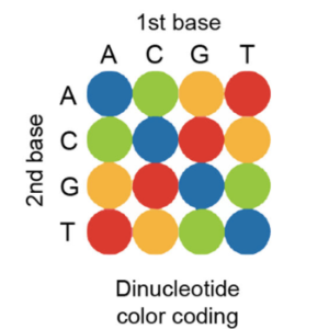
In SOLiD sequencing-by-ligation, critical enzymatic steps can be performed directly on a standard microscope at room temperature. First, a sequencing primer is hybridized to multiple copies of the adapter sequence in RCA amplicons, followed by ligation of dinucleotide-specific fluorescent oligonucleotides. After imaging, the fluorophores are cleaved from the ligation complex, and ligation of fluorescent oligonucleotides is repeated six more times to interrogate dinucleotide pairs at every fifth position (Fig.1 b). To fill in the gaps between dinucleotide pairs, the whole ligation complex is stripped off, and four additional sequencing primers with a single base offset are used to repeat dinucleotide interrogation starting from positions n-1, n-2, n-3 and n-4, generating up to 35 raw 3D image stacks representing dinucleotide compositions at all base positions over time.
The raw images are enhanced using standard 3D deconvolution techniques to reduce the background noise, and our MATLAB script performs image alignment to produce TIFF images that are then used for base calling using a separate Python script. The base calls from individual pixels are then aligned to the reference transcriptome using Bowtie, and neighboring pixels with highly similar sequences are grouped into a single object generating a consensus sequence. The final dataset includes the number of individual pixels per object, gene ID, consensus sequence, x and y centroid positions, number of mismatches, base call quality and alignment quality.
One of the key considerations early in the development of FISSEQ was imaging. Biological patterns, including RNA localization, occur in a scale-dependent manner, in which some patterns are visible at one scale but disappear at another. Therefore, we developed our sequencing method specifically for confocal microscopy using a wide range of objectives, magnification, numerical apertures, scanning speed and depth. Also, autofluorescence, cell debris, and background noise are common in cell imaging, unlike in standard Next-generation sequencing. So we developed an approach to classify individual pixels based on their specific color transitions to detect true signals even in the noisy and/or low intensity environment. Finally, we also developed a way to control the imaging density of single molecules, enabling one to sequence the sequence a large number of molecules in single cells regardless of the microscopy resolution.
Applications
The current FISSEQ protocol is suitable for most cultured cells and tissue sections, including formalin-fixed and paraffin-embedded (FFPE) tissue sections. Whole mount Drosophila embryos, iPS-cell derived embryo bodies (EBs) and organoids are also compatible (Table 1). In FISSEQ each sequencing read has a spatial coordinate, and the reads are binned according to the cellular morphology, sub-cellular location, protein localization, or GFP fluorescence. A statistical test is then applied to identify enriched genes and pathways de novo and discover possible biomarkers of the cellular phenotype23. This approach may be combined with padlock probes to detect evolving mutations and RNA biomarkers in cancers12,13 or to compare gene expression in asymmetric cells or tissues.
FISSEQ may also sequence molecular barcodes in individual cells and transcripts, where expression or reporter (i.e. cDNA, promoter-GFP) libraries are examined in a pool of single cells for massively parallel functional assays and cell lineage tracing. In essence a practically unlimited number of DNA-associated cellular features may now be imaged, enumerated and analyzed across multiple spatial scales using the DNA sequence as a temporal barcode.
Limitations
On a practical level, equipping a microscope for four-color imaging can cost up to $20,000 for a new filter set and a laser. Most users will need to reserve the microscope for 2–3 weeks so that sequencing can proceed uninterrupted. We have used laser scanning confocal, wide-field epifluorescence and spinning disk confocal microscopes and obtained comparable sequencing data that differ mainly in the read density. With the laser scanning confocal microscope, imaging can take over 30 minutes per stack, but wide-field or spinning disk confocal microscopes can image the same volume in 1–2 minutes. Reagent exchanges are done manually in the current protocol, but FISSEQ samples can remain on the microscope and be sequenced over 2–3 weeks.
On a technical level, a major limitation of our current protocol is the lack of ribosomal RNA depletion. Initially we used ribosomal RNA as an internal control for library construction, sequencing and bioinformatics; however, this reduced the number of mRNA reads per cell. In primary fibroblasts the ribosomal RNA reads comprised 40–80% of the total23; therefore, if one were to deplete the ribosomal RNA24, it may be possible to increase the number of mRNA reads per cell by ~5 fold.
Another limitation is the lack of information on biases in our method. FISSEQ enriches for biologically active genes, enabling discrimination of cell type-specific processes with a small number of reads23; however, it is not clear how such enrichment occurs. We hypothesize that active RNA molecules are more accessible to FISSEQ, whereas RNA molecules involved in ribosome biogenesis, RNA splicing, or heat-shock response are trapped in ribonucleoproteins, spliceosomes, or stress granules. It is now important to investigate and understand the molecular basis of such enrichment across multiple cell types and conditions and correlate the result with the observed cellular phenotype.
Experimental design
General considerations—This protocol details the method described in our original report23, where endogenous RNAs in cultured fibroblasts were sequenced on a confocal microscope. The availability of a microscope and computational resources will guide the general experimental approach (Table 2). We provide basic computational tools along with a sample dataset, but a background in python, MATLAB, ImageJ and/or R is helpful for analyzing a large number of images. If such expertise is not available, we recommend focusing on a few regions-of-interest with well-demarcated features for comparing gene expression using our custom scripts23. After outlining the experiment, one should download our sample image, software and dataset and become familiar with image and data analysis (http://arep.med.harvard.edu/FISSEQ_Nature_Protocols_2014/). One should then finalize the experimental design and define the imaging parameters (i.e. area, thickness, resolution, magnification).
Cell and tissue fixation—We have been able to fix and generate in situ sequencing libraries in a wide number of biological specimens (Table 1). The only case in which we failed was a hard piece of bone marrow embedded in Matrigel, which detached from the glass surface after several wash steps. Fixation artifacts can include changes in sub-cellular RNA localization, cell swelling, incomplete permeabilization and RNA leakage. Certain primary cell types are also sensitive to cold42, while transformed cell lines or stem cells appear to be less sensitive (Fig. S1). If using FISSEQ to study sub-cellular localization, we recommend fixing cells by adding warm formalin directly into the growth media to a final concentration of 10%.
Cell and tissue sample mounting—For high resolution imaging we recommend poly lysine- or Matrigel-coated glass bottom dishes, but 96-well plastic bottom plates can be used for simple protocol optimization. Tissue sections can be mounted using a standard mounting procedure, and we advise inexperienced users to consult those practiced in the art of tissue mounting. For non-adherent cell types and whole mount specimens, we recommend fixing samples embedded in Matrigel using 4% paraformaldehyde on a glass bottom dish.
Reverse transcription (RT) in situ—The length of RT primers should be less than 25 bases to prevent self-circularization. We perform RT overnight for most samples, but one hour is often sufficient for cell monolayers. A negative control without RT should be included to rule out self-circularization of the primer. A positive control primer with the adapter sequence plus a synthetic sequence (~30 additional bases) can be used to check rolling circle amplification (RCA) and imaging parameters. Other than the 5’ region of highly abundant mCherry transcripts23, we have not had consistent results with targeted RT. We typically see very few amplicons regardless of the primer design, while random hexamers (24 bases) and poly dT primers (33 bases) work well across all conditions. Some of the possible reasons for failure may include poor target accessibility and competitive inhibition of CircLigase by non-specifically bound sequence-specific RT primers capable of self-circularization. Possible solutions include using LNA-based RT primers for high temperature hybridization13, ligation of the adapter sequence post-RT and tiling multiple RT probes across a gene target. We have yet to try these alternatives.
Generation of amplicon matrix—Aminoallyl dUTP is a dTTP analog commonly used in fluorescence labeling of cDNA43, which we utilize for cross-linking nucleic acids; however, the efficiency of RT and RCA is inversely correlated with the concentration of aminoallyl dUTP23. The cross-linker, bis(succinimidyl)-nona-(ethylene glycol) or BS(PEG)9, is functionalized with NHS ester groups at both ends44, and it forms a stable covalent bond with primary amine groups provided by aminoallyl dUTP at pH 7–9. The cross-linking density can be enhanced by increasing the concentration of aminoallyl dUTP or BS(PEG)9, or by increasing the pH. Cross-linking after RT is optional, but cross-linking of RCA amplicons is essential for high quality sequencing reads.
Sequencing—We use sequencing-by-ligation18, 19, 45 (SOLiD46, 47) because it works well at room temperature and so a heated stage is not required. SOLiD uses a dinucleotide detection scheme where a base position is interrogated twice per sequencing run46, 47, and this can reduce the base calling error rate; however, converting the color sequence to the base sequence is not straightforward due to its propensity to propagate errors, and sequence analysis must remain in the color space (Box 1). In comparison, sequencing-by-synthesis (Illumina) works at 65°C for primer extension and cleavage and utilizes proprietary fluorophores, requiring a heated flow-cell and a custom imaging set-up. Since sequencing-by-synthesis can generally yield a much longer read length, we are currently investigating its compatibility with FISSEQ.
Partition sequencing—T4 DNA ligase has a single-base specificity at the ligation junction18, and sequencing primers differing by one base can recognize different sets of amplicons23. By dividing imaging over multiple separate runs, spatially overlapping amplicons can be enumerated using multiple sequencing primers even on a low resolution microscope; however, this requires full automation for the increased number of sequencing runs per sample. Without automation partition sequencing is better suited for quantifying short barcode sequences rather than full RNA sequences in situ12 (Fig. 3).
Imaging—Epifluorescence microscopy can generate a reasonable number of alignable reads from relatively thin specimens (<5-um), such as HeLa cells23, but thicker samples require confocal microscopy to obtain high density reads. Spinning disk confocal microscopy is significantly faster than laser scanning confocal microscopy, and it has a good balance of imaging speed and axial resolution. An automated stage capable of finding a z-stack across multiple x-y tiles is highly desirable (Table 2).
In FISSEQ individual amplicons can be detected using objectives with N.A. 0.4 or greater. The magnification required is determined by the biological question and the amplicon density48. Typically we use a 20× N.A. 0.75 objective to examine tissue sections and cultured cell mono-layers, while 40× N.A. 0.8 and 63× N.A. 1.2 water immersion objectives are used for high-resolution imaging of single cells. We have observed noticeable chromatic aberration in our experiments, depending on the objectives used. The degree of chromatic aberration should be measured using image calibration beads (i.e. FocalCheck Fluorescence Microscope Test Slide) prior to sequencing and calibrated by the microscope vendor if necessary.
For each imaging set-up the user should determine the ideal Nyquist rate. This value can be calculated using http://www.svi.nl/NyquistCalculator. The x-y pixel and z-step sizes should not be greater than 1.7 times the Nyquist value for image deconvolution. Four color imaging should proceed from the longest to shortest wavelength (i.e. Cy5, Texas Red, Cy3, FAM), and an intensity histogram should be used to adjust laser power to prevent saturated pixels. The intensity histogram should be consistent across fluorescence channels and sequencing cycles. To use our software the image file name must be standardized: <Position>_<Primer #>_ <Ligation #>_<Date_Time>.extension (e.g. 06_N1_2_2013_10_25_11_57_18.czi).
Image analysis tools—In practice the extent of image processing and analysis is dictated by the available imaging tools and computing resources49. We use Bitplane Imaris for data visualization and movie creation and SVI Huygens for 3D deconvolution. While they are easy to use, scalable and relatively fast, their cost may be out of reach for small labs; however, free and/or open source alternatives are also available49–51.
Image deconvolution—We use 3D deconvolution52 to reduce the out-of-focus background and improve the quality of base calls (Fig. 5a). High quality 3D deconvolution requires sampling near the Nyquist rate, but this increases the image acquisition and deconvolution time as well as the file size. We generally recommend using high-quality confocal imaging and minimal 3D deconvolution for FISSEQ. Using 3D deconvolution to compensate for low quality imaging will not necessarily improve the quality or number of sequencing reads. We provide a sample dataset containing raw and deconvolved image stacks from a successful 30-base sequencing experiment for practice (http://arep.med.harvard.edu/FISSEQ_Nature_Protocols_2014/).
Image registration, base calling and sequence alignment—As long as the input image files are correctly named, our software will generate the maximum intensity projection, register images and correct for chromatic shifts23 (Fig. 5b). The resulting images are used for base calling and sequence alignment to human RefSeq (Fig. 5c), but our software does not generate z-coordinates for sequencing reads, as it uses maximum intensity projection for base calling. We provide a sample data output and screen logs for troubleshooting our bioinformatics software (http://arep.med.harvard.edu/FISSEQ_Nature_Protocols_2014/).
Data analysis—Our software generates a tab delimited text file containing 10,000 to 50,000 aligned reads per field of view. We recommend RStudio with the latest version of R installed for plotting reads by RNA classes, position, cluster size, quality, gene name, strand, etc. We provide a sample R session file used for FISSEQ data analysis as an introduction to statistical computing and assessing the quality of FISSEQ dataset (http://arep.med.harvard.edu/FISSEQ_Nature_Protocols_2014/).
Level of expertise required for the protocol—FISSEQ is at the interaction of cell imaging and functional genomics, and it has generated much interest from cell biologists not familiar with RNA-seq. Our protocol is aimed at such researchers, who are familiar with cell image analysis but have few computing skills (Fig. 6). FISSEQ library construction can be performed by anyone with basic molecular biology skills, but image acquisition is best done with help from an imaging core specialist for the initial set-up. Once the equipment, software, imaging and deconvolution parameters are finalized, a capable technician, graduate student, or post-doc can perform manual sequencing on a microscope with some training and practice. Image and sequence analysis using our software can be performed by anyone familiar with the Unix environment, but statistical data analysis requires either a graduate student or post-doc familiar with statistical tools and concepts.
Considerations about the laboratory facilities—All steps in FISSEQ library construction can be carried out in a standard laboratory setting. A vacuum line facilitates solution aspiration and reagent exchanges, and we do not find RNA degradation or PCR contamination to be a significant problem in our method. We advise having a dedicated microscope with proper excitation and emission filters on a vibration isolation table in a low traffic area.
TROUBLESHOOTING
Supplementary Material
Refer to Web version on PubMed Central for supplementary material.
Acknowledgments
Funded by NIH CEGS grant P50 HG005550. J.H.L. and coworkers funded by NHBLI grant RC2HL102815, Allen Institute for Brain Science, and NIMH grant MH098977. E.R.D. funded by NIH grant GM080177 and NSF GRF grant DGE1144152.
For additional information and references please see the attached full manuscript.
Materials
MATERIALS
Starting material of interest. The Procedure is written for cultured cells in glass bottom dishes or for tissue sections on glass bottom dishes or cover slips. However, it can be adapted for use on a range of starting materials (see Table 1 in Guidelines).
Acetone (for detaching a Petri dish glued to the microscope stage)
Aminoallyl dUTP, 4 mM (Anaspec, part no. 83203)AnaspecCatalog #83203
Betaine, 5 M (included in CircLigase II kit)EpicentreCatalog #CL9025K
BS(PEG)9, 100 mg (Note: BS(PEG)9 loses its effectiveness 1 month after reconstitution in DMSO. Prepare a fresh batch every month, especially if it has been frozen and thawed repeatedly.Thermo ScientificCatalog #21582
CircLigase II kit EpicentreCatalog #CL9025K
Cleave Solution 1 Applied Biosystems (ThermoFisher Scientific)Catalog #4406489
Cleave Solution 2.1 KitApplied Biosystems (ThermoFisher Scientific)Catalog #4445677
Cyanoacrylate adhesive, optical grade VWR International (Avantor)Catalog #19806-00-1
DEPC-treated water Santa Cruz BiotechnologyCatalog #sc-204391
DMSO Merck MilliporeSigma (Sigma-Aldrich)Catalog #D8418
dNTP, 25 mM EnzymaticsCatalog #N2050L
Ethanol, 70% (in DEPC water)
Formalin, 10% Electron Microscopy SciencesCatalog #15740
Formamide Merck MilliporeSigma (Sigma-Aldrich)Catalog #221198
HCl, 0.1 N (in DEPC water)
Immersol W 2010 (ne=1.33) for water immersion lens ZeissCatalog #444969-0000-000
Instrument Buffer, 10XApplied Biosystems (ThermoFisher Scientific)Catalog #4389784
M-MuLV reverse transcriptase EnzymaticsCatalog #P7040L
Mineral oil Merck MilliporeSigma (Sigma-Aldrich)Catalog #M5904
MnCl2 (included in CircLigase II kit)EpicentreCatalog #CL9025K
Nuclease-free water, not DEPC-treated Life TechnologiesCatalog #AM9932
Pepsin, 1 g (dissolve in 10 ml H2O and store at −20°C)AffymetrixCatalog #20010
Phi29 DNA polymeraseEnzymaticsCatalog #P7020-HC-L
Phosphate-buffered solutionLife TechnologiesCatalog #10010023
RNase, DNase-freeRocheCatalog #11579681001
RNase H EnzymaticsCatalog #Y9220F
RNase inhibitor EnzymaticsCatalog #Y9240L
RNaseZap Life TechnologiesCatalog #AM9780
Silicone isolator Grace Bio-LabsCatalog #664304
Sodium acetate, 3 M (pH 7.5)
SOLiD™ ToP Sequencing Kit Fragment Library F3 Tag MM50Applied Biosystems (ThermoFisher Scientific)Catalog #4449388
SSC, 20XRocheCatalog #11666681001
Streptavidin Alexa Fluor 647 Life TechnologiesCatalog #S32357
T4 DNA ligase EnzymaticsCatalog #L6030-LC-L
Tris solution, 1 M G-BiosciencesCatalog #R002
Trisodium citrate dihydrate Merck MilliporeSigma (Sigma-Aldrich)Catalog #C8532
Triton X-100, 10% solution Merck MilliporeSigma (Sigma-Aldrich)Catalog #93443
RT, RCA and SEQUENCING PRIMERS are listed in Guidelines
CONTROL PRIMERS are listed in Guidelines
EQUIPMENT is listed in Guidelines
Troubleshooting
Safety warnings
- Acetone is highly flammable. Work in a well-ventilated area.
- Cleave Solution 2.1 Kit contains toxic organoamine. Wear gloves and work in a well-ventilated area.
- When handeling Formalin, 10% wear gloves and work in a well-ventilated area. Dispose of waste per institutional guideline.
- The Flexible plastic I.V. catheter for reagent aspiration comes with a plastic outer sheath and a sharp needle in the middle. The needle must be carefully removed and discarded into a sharps container.
Before start
REAGENT SETUP
0.25% Triton X-100 Dilute 0.25 ml 10% Triton X-100 in DEPC-treated H2O to a total volume of 10 ml. Store at RT for 6 months.
2X SSC Dilute 20X SSC in H2O and make up to a total volume of 50 mL. Store at RT for 6 months.
1X SSC Dilute 20X SSC in H2O and make up to a total volume of 50 mL. Store at RT for 6 months.
5X SASC Make 0.75 M sodium acetate, 75 mM tri-sodium citrate, pH to 7.5 using acetic acid in H2O to a final volume of 50 ml. Store at RT for 6 months.
RCA primer hybridization buffer Dilute 20X SSC2x SASC, 30% formamide in H2O. Store at RT for 6 months.
Strip Buffer (80% formamide in H20, 0.01% Triton-X100 in a final volume of 50 ml. Store at RT for 6 months.
Cleave Solution 2.1, reconstituted Mix 1 ml Cleave Solution 2.1 Part 1 with 2.75 ml Cleave Solution 2.1 Part 2. Store at 4°C in dark for up to 24 hours.
EQUIPMENT SETUP
Microscope setup—Configure a 4 channel microscope with appropriate excitation light sources and emission filters: FITC-488 ex, 490–560 nm em; Cy3–561 nm ex, 563–593 nm em; Texas Red-594 nm ex, 597–647 nm em; Cy5–633 nm ex, 637–758 nm em. Suggested microscope objectives are Plan-Apochromat dry 20× NA 0.75, dry 40× NA 0.8 and water immersion 63× NA 1.3.
Software installation—Verify that Bio-Formats (http://loci.wisc.edu/software/bio-formats) plug-ins are available for Fiji/ImageJ. Download a free academic version of Canopy Python 2.7 (https://www.enthought.com/downloads) in the home directory on the remote host, and follow the installation instruction (http://docs.enthought.com/canopy/quick-start/install_linux.html). Canopy Python 2.7 is easy to install and has all the required packages for our FISSEQ software. Install the latest version of ggplot2 and data.table packages in RStudio.
PC setup
- Access to a high performance computing cluster (remote host)
- Bowtie 1.0 or earlier (http://bowtie-bio.sourceforge.net) on the remote host CRITCAL Bowtie 2.0 or higher does not work with SOLiD sequencing.
- Python 2.7 (https://www.enthought.com/products/canopy/) on the remote host CRITCAL Other versions of Python lack the required modules for running our script.
- Windows PC or Mac with 16GB RAM minimum
- Optional: SVI Huygens 3D deconvolution software (commercial), Bitplane Imaris 3D rendering software (commercial)
FISSEQ library construction in cultured cells or tissue sections
This step can be performed using option A or B depending on the type of a specimen examined. All reagents and washes are at RT unless indicated otherwise.
Option B: Tissue sections on a glass bottom dish.
TROUBLESHOOTING
Prepare a reverse transcription mixture on ice, as indicated below.
Note
CRITICAL STEP Chilling the assembled mix to 4°C prior to RT improves the efficiency of primer annealing.
159 µL DEPC-H2O
20 µL M-MuL V RT buffer, 10x
2 µL dNTP, 25 mM
2 µL Aminoallyl dUTP, 4 mM
5 µL RT primer, 100 μM (/5Phos/TCTCGGGAACGCTGAAGANNNNNN)
2 µL RNase Inhibitor (40 U μl−1)
10 µL M-MuLV reverse transcriptase (100 U μl−1)
Incubate the specimen with the reaction mixture for 10 min at 4°C, then transfer to 37°C overnight. Typically 1–2 hours is sufficient, but more time may be required for thicker samples. Aspirate and wash with PBS once.
TROUBLESHOOTING
4 °C Incubation
00:10:00 Incubation at 4°C
37 °C Incubation overnight
To cross-link cDNA molecules containing aminoallyl dUTP, add 20 μl reconstituted BS(PEG)9 in 980 μl PBS to sample for 1 hr at RT.
980 µL PBS
20 µL Reconstituted BS(PEG)9
980 µL PBS
01:00:00 Incubation at RT
Aspirate and wash with PBS and quench with 1 M Tris pH 8.0 for 30 min.
Note
PAUSE POINT The sample can be stored in PBS for up to a week at 4°C.
00:30:00 PBS wash
Aspirate and add 10 μl DNase-free RNase and 5 μl RNase H in 1× RNase H buffer for 1 hr at 37°C (Figure).
Note
CRITICAL STEP Skipping this step results in few amplicons.
10 µL DNase-free RNase
5 µL RNase H in 1× RNase H buffer
37 °C Incubation
01:00:00 Incubation
Rinse with 2 ml nuclease-free H2O twice to remove traces of phosphate.
TROUBLESHOOTING
2 µL Nuclease-free H2O
Prepare a CircLigase reaction mixture on ice as tabulated below, and add to the glass bottom dish containing fixed cells.
20 µL CircLigase buffer, 10×
10 µL MnCl2, 50 mM
40 µL Betaine, 5 M
2 µL CircLigase II (100 U μl−1)
128 µL Nuclease-free H2O
20 µL CircLigase buffer, 10×
10 µL MnCl2, 50 mM
2 µL CircLigase II (100 U μl−1)
40 µL Betaine, 5 M
Place the glass bottom dish in a tightly sealed plastic container or a Ziploc bag with moist wipes and incubate at 60°C for 1 hr. If a longer reaction time is desired, 1 ml of mineral oil can be layered on top of the cells.
60 °C Incubation
01:00:00 Incubation
1 µL Mineral oil (optional)
Aspirate the reaction mixture, and wash with PBS. Mineral oil can be removed using PBS with 0.1% Triton X-100.
Note
PAUSE POINT The sample can be stored in PBS at 4°C indefinitely.
Add 200 μl RCA primer hybridization buffer containing 500 nM RCA primer to the glass bottom dish and incubate at 60°C for 1 hr.
200 µL RCA primer hybridization buffer containing 500 nM RCA primer
60 °C Incubation
01:00:00 Incubation
Aspirate and wash with RCA hybridization buffer at 60°C for 10 min.
60 °C Wash with RCA hybridization buffer
00:10:00 Wash with RCA hybridization buffer
Aspirate and wash with 2X SSC, 1X SSC and PBS once each.
Prepare an RCA reaction mixture on ice as tabulated below. Add to the sample and incubate overnight at 30°C. Additional dNTP (up to 10 μl) and Phi29 DNA polymerase (up to 10 μl) can enhance the fluorescence signal from DNA amplicons.
| Component | Amount (µl) | Final | |
| Nuclease-free H2O | 174 | ||
| Phi29 buffer, 10x | 20 | 1 x | |
| dNTP, 25 mM | 2 | 250 µM | |
| Aminoallyl dUTP, 4 mM | 2 | 40 µM | |
| Phi29 DNA polymerase (100 U µl-1) | 2 | 1 U µl-1 | |
| Total | 200 |
Note
CRITICAL STEP Aminoallyl dUTP is required for cross-linking and should not be omitted.
174 µL Nuclease-free H2O
20 µL Phi29 buffer, 10x
2 µL dNTP, 25 mM
2 µL Aminoallyl dUTP, 4 mM
2 µL Phi29 DNA polymerase (100 U µl-1)
To cross-link cDNA molecules containing aminoallyl dUTP, wash gently with PBS, add 20 μl reconstituted BS(PEG)9 in 980 μl PBS to sample and incubate for 1 hr at RT.
Note
CRITICAL STEP BS(PEG)9 expires after 2–3 wks with multiple freeze-thaw cycles, and using expired BS(PEG)9 can lead to unstable amplicons and poor sequencing results.
20 µL reconstituted BS(PEG)9
980 µL PBS
01:00:00 Incubation at RT
Wash with PBS, aspirate and add 1 M Tris pH 8.0 for 30 min.
Note
PAUSE POINT Store in PBS at 4°C for up to 4 weeks.
00:30:00 Incubation
Aspirate and add 2.5 μM control probe in 200 μL 5X SASC, pre-heated to 80°C, to the sample and incubate for 10 minutes at RT. Use the adapter- or ribosomal RNA-specific probes to image all or rRNA amplicons respectively. RT-negative controls should not produce any amplicons.
200 µL 5X SASC
80 °C 5X SASC
00:10:00 Incubation at RT
Wash two times for 1 minute each with 1 mL 1X Instrument Buffer. If using adapter sequence-specific probe, proceed directly to Step 19 for imaging. If using the biotinylated ribosomal RNA probes, incubate in 2 μg ml−1 Streptavidin Alexa Fluor in PBS for 5 min, followed by three 2 ml PBS washes before continuing with Step 19.
00:01:00 Wash (1/2)
00:01:00 Wash (2/2)
2 µL 1X Instrument Buffer
00:05:00 Incubation in Streptavidin Alexa Fluor in PBS (optional)
6 µL PBS (optional)
Image on a microscope and inspect the amplicon density and distribution. Amplicons should be distributed uniformly throughout the sample across the glass bottom dish. Obtain an axial view and check to see if the amplicon density is similar between regions near the glass and cell surface.
Note
CRITICAL STEP The sample can be imaged while immersed in 1X Instrument Buffer. If alternative immersion liquid is used, do not add Tris-EDTA or other chelating agents.
Aspirate and incubate two times for 5 minutes each in 1 mL Strip Buffer at RT, pre-heated to 80°C.
2 µL Strip Buffer
00:05:00 Incubation (1/2)
00:05:00 Incubation (2/2)
80 °C Strip Buffer
Wash two times for 5 minutes each with 1 mL 1X Instrument Buffer at RT.
Note
PAUSE POINT We have kept samples in 1X Instrument Buffer at 4°C for up to several months without suffering a significant loss in the fluorescence signal.
2 µL 1X Instrument Buffer
00:05:00 Wash (1/2)
00:05:00 Wash (2/2)
SOLiD sequencing-by-ligation
Clamp the sample firmly to the microscope stage, and use cyanoacrylate adhesive to secure any potential sources of movement, such as adjustable stage inserts. Cyanoacrylate adhesive can be applied directly to metal components and removed with acetone after sequencing.
Note
CRITICAL STEP Use only optical-grade cyanoacrylate adhesive, as standard cyanoacrylate adhesives de-gas and ruin nearby objectives.
Add 2.5 μM sequencing primer N in 200 μL 5X SASC, pre-heated to 80°C, to the sample and incubate for 10 minutes at RT. Aspiration can be performed using a vacuum aspirator or a flexible plastic catheter attached to a syringe.
2.5 µL Sequencing primer N
200 µL 5X SASC
80 °C 5X SASC
00:10:00 Incubation at RT
Wash two times for 1 minute each with 1 mL 1X Instrument Buffer at RT.
2 µL 1X Instrument Buffer
00:01:00 Wash (1/2)
00:01:00 Wash (2/2)
Sequence the sample by adding a freshly prepared T4 DNA ligation mixture and incubating for 45 minutes at RT.
165 µL Nuclease-free H2O
20 µL T4 DNA ligase buffer, 10×
10 µL T4 DNA ligase, 120 U μl−1
5 µL SOLiD sequencing oligos (dark purple tube from the SOLiD ToP sequencing kit)
00:45:00 Incubation
Wash four times for 5 minutes each with 1 mL 1X Instrument Buffer at RT.
4 µL 1X Instrument Buffer at RT
00:05:00 Wash (1/4)
00:05:00 Wash (2/4)
00:05:00 Wash (3/4)
00:05:00 Wash (4/4)
Acquire images.
Note
CRITICAL STEP The first ligation cycle for recessed primers N-2, N-3 and N-4 produces a fluorescence signal in just one channel. These images should NOT be included in the final dataset.
Aspirate and cleave the fluorophore by incubating the sample two times for 5 minutes each in Cleave Solution 1 and then two times for 5 minutes each in reconstituted Cleave Solution 2.1 mix at RT.
00:05:00 Incubation in Cleave Solution 1 (1/2)
00:05:00 Incubation in Cleave Solution 1 (2/2)
00:05:00 Incubation in reconstituted Cleave Solution 2.1 mix (1/2)
00:05:00 Incubation in reconstituted Cleave Solution 2.1 mix (2/2)
Aspirate and wash three times for 5 minutes each with 1 mL 1X Instrument Buffer.
3 µL 1X Instrument Buffer
00:05:00 Wash (1/3)
00:05:00 Wash (2/3)
00:05:00 Wash (3/3)
Note
PAUSE POINT The sample is stable for 2–3 days in 1X Instrument Buffer at RT.
Go to Step 25 and repeat 6 times for a total of 7 cycles.
Repeat cycle
Incubate four times for 5 minutes each in 1 mL Strip Buffer, pre-heated to 80°C.
4 µL Strip Buffer
80 °C Strip Buffer
00:05:00 Incubation (1/4)
00:05:00 Incubation (2/4)
00:05:00 Incubation (3/4)
00:05:00 Incubation (4/4)
Wash two times for 1 minute each with 1 mL 1X Instrument Buffer.
Note
PAUSE POINT The sample is stable for 2–3 days in 1X Instrument Buffer at RT.
2 µL 1X Instrument Buffer
00:01:00 Wash (1/2)
00:01:00 Wash (2/2)
Repeat steps 23–32 using different sequencing primers (N-1, N-2, N-3, and N-4).
Repeat steps 23-32
If necessary use ImageJ to crop image stacks for faster 3D deconvolution.
Determine optimal 3D deconvolution parameters using a smaller cropped test image from the experiment. In Huygens Professional we typically use a Nyquist sampling rate of 1.7, CMLE mode, 5–10 iterations and a signal-to-noise ratio of 2–5.
Deconvolve all sequencing images, and save images as .ics/.ids files with the following names in a folder named ‘decon_images’ (Figure).
Filename: <Position>_<Primer #>_<Ligation #>_<Date__Time>.<ext>
Position: Dinucleotide position as 2-digit integers 01 to 30
Primer number: N followed by 1-digit integers N0 to N4
Cycle number: Ligation cycle per primer from 1 to 7
Date/time: An alphanumeric string using underscores
File extension: .ics and .ids
TROUBLESHOOTING
Image analysis
Download fisseq.zip (http://arep.med.harvard.edu/FISSEQ_Nature_Protocols_2014/) and copy to a remote host using a command line terminal on a PC.
Note
CRITICAL Some users of our method may have little or no background in bioinformatics. Here we introduce common computational environment and tools, but novice users should obtain additional help from experienced users, network administrators and online resources (i.e. http://www.ee.surrey.ac.uk/Teaching/Unix/).
Command
Download and unzip decon_images.zip (http://arep.med.harvard.edu/FISSEQ_Nature_Protocols_2014/). Copy decon_images folder (Step 36) to a scratch space on the remote host.
Command
Logon to the remote host, and submit a job request to work on a high memory queue interactively. We recommend at least 100GB (mem below is in MB).
Command
Unzip fisseq.zip, and change the working directory to fisseq.
Command
Note
CRITICAL STEP Working from folders other than ~/fisseq results in missing file errors when entering our commands as written below.
Download and decompress the RefSeq-to-Gene ID conversion table.
Command
Download the organism-specific RefSeq RNA FASTA file, and unzip the file.
Command
Build the reference index of [ref_name] in color space. Here [ref-name] is refseq_human. This process can take several hours.
TROUBLESHOOTING
Command
Start MATLAB, and add a search path:
Command
Define the input and output directories and run image registration (Figure).
Number of blocks per axis for local registration (default = 10)
Fraction overlap between neighboring blocks (default = 0.1)
Alignment precision where 10 will register images to 1/10 of a pixel. (default = 1)
TROUBLESHOOTING
Command
Copy files in ~/fisseq/registered_images/ to a PC. Use ImageJ to open TIFF files (File > Import > Bio-Formats) as a time series, and check alignment in channel 4 by scrolling through the timeline (Supplementary Movies 1–4).
Maximum-projected TIFF files (channel 4 is a composite of channel 0 to 3).
Routput.mat: Block-wise registration offsets between bases.
Rchadj.mat: Block-wise chromatics shifts as a matrix.
Rtadj.mat: Registration offsets over time for the whole image (not block-wise).
TROUBLESHOOTING
Start Python, and write base calls to read_data_*.csfasta. The maximum number of missing base calls allowed per read is 6 by default. * denotes an automatically generated time stamp.
TROUBLESHOOTING
Command
Align reads to refseq_human (Step 43) using Bowtie 1.0 or earlier, and write mapped reads to bowtie_output.txt. The exact name of read_data_*.csfasta can be determined by listing files in the directory (ls -l).
Command
Spatially cluster the Bowtie reads (Step 48), annotate clusters using gene2refseq (Step 41) and write to results.tsv. The default kernel size of 3 performs a 3×3 dilation prior to clustering.
Command
Data analysis
Open the FISSEQ RStudio project file (Menu > File > Open project…).
Note
CRITICAL Data analysis can be done on any software package, but R is convenient for interactive analysis and high-quality graphs23. Novice users may find RStudio more intuitive than the command line interface. We provide a sample R session containing a sample dataset and a list of commands (http://arep.med.harvard.edu/FISSEQ_Nature_Protocols_2014/).
Find the HISTORY tab on the upper right console window and double-click on individual commands in order to re-execute the previous R session (Fig. S6) and learn how to:
Import and filter data using a specific criterion (i.e. cluster size)
Plot a distribution of reads by a specific criterion (i.e. RNA classes and strands)
Convert a table of reads into a table of gene expression level
Correlate gene expression from different images
Find statistically enriched genes in different regions
TROUBLESHOOTING
Troubleshooting advice can be found in Table 3 (Guidelines).