Sep 26, 2025
Fibroblast/ECM Functional Units: A Medium-Throughput Assay and Digital Analysis Pipeline V1
- Aleksandr Dolskii1,
- Ekaterina Shitik2,
- Mariia Dmitrieva1,
- Olivia Williams1,
- Glenn Ma1,
- Tiffany Luong1,
- Janusz Franco-Barraza1,
- Edna Cukierman3,
- Michael Miano4
- 1Cancer Signaling & Microenvironment Program, M&C Greenberg Pancreatic Cancer Institute, Fox Chase Cancer Center, Lewis Katz School of Medicine, Temple Health, Philadelphia, PA 19111, United States;
- 2Independent researcher, Novi Sad, Serbia;
- 3Fox Chase cancer center / Temp;
- 4Fox Chase Cancer Center
- Aleksandr Dolskii: [email protected];


Protocol Citation: Aleksandr Dolskii, Ekaterina Shitik, Mariia Dmitrieva, Olivia Williams, Glenn Ma, Tiffany Luong, Janusz Franco-Barraza, Edna Cukierman, Michael Miano 2025. Fibroblast/ECM Functional Units: A Medium-Throughput Assay and Digital Analysis Pipeline V1. protocols.io https://dx.doi.org/10.17504/protocols.io.e6nvwqyz7vmk/v1
License: This is an open access protocol distributed under the terms of the Creative Commons Attribution License, which permits unrestricted use, distribution, and reproduction in any medium, provided the original author and source are credited
Protocol status: Working
We use this protocol and it's working
Created: May 19, 2025
Last Modified: September 26, 2025
Protocol Integer ID: 218562
Keywords: Extracellular matrix, ECM, Cancer-associated fibroblasts, CAFs, Fibroblasts, Fibroblast/ECM functional unit, Cell-derived matrix, CDM, Tissue microenvironment, Pancreatic ductal adenocarcinoma, PDAC, pancreatic cancer, Cell–matrix interactions, Fibrillogenesis, Fibrosis, Wound healing, Fibroblast activation, Matrix-induced functions, Cell-adhesion signaling, Confocal, imaging analysis, Image post-processing, Fibronectin fiber alignment, Nuclei segmentation, StarDist, Orientation analysis, OrientationJ, OrientationPy, Fiji, ImageJ, digital analysis pipeline v1 fibroblasts secrete, characterization of fibroblast, associated fibroblast, fibroblast, extracellular matrix, structural support for cell adhesion, ecm functional unit, pancreatic ductal adenocarcinoma, cell adhesion, derived cancer, wound healing, including ecm thickness, biomedical research
Funders Acknowledgements:
NIH
Grant ID: R01CA269660
NIH
Grant ID: U54CA272686
NIH equipment grant
Grant ID: S10ODO23666
DOD grant
Grant ID: HT9425-23-1-0584
ACS Wilmott Family Pancreatic Cancer Professorship
Grant ID: RP-23-1070169-01-WRP
NIH/NCI Comprehensive Cancer Center Core Grant
Grant ID: P30CA06927
Abstract
Fibroblasts secrete and organize the extracellular matrix (ECM), which provides structural support for cell adhesion, migration, and tissue architecture, while also regulating critical cellular functions such as growth and survival (see DOI: 10.1152/physiolgenomics.00158.2013 and DOI: 10.1158/0008-5472.CAN-24-2860). Studying these fibroblast-dependent features is crucial across various areas of biomedical research, including cancer and wound healing. In this protocol, we use patient-derived cancer-associated fibroblasts (CAFs) from pancreatic ductal adenocarcinoma (PDAC) patients due to the crucial role of desmoplasia in the disease. A widely used model system is the fibroblast/ECM functional units (see DOI: 10.1016/bs.mcb.2019.11.014), a multilayered structure consisting of fibroblasts and their self-produced ECM. This protocol optimizes the generation of such units on glass slides using silicone isolators that create 12 independent wells, significantly increasing throughput. It also supports production in standard 96-well plates. Both formats reduce sample consumption per reaction while expanding the number of test conditions per experiment, whether for condition effect screening or evaluating the role of specific genetic modifications. Characterization of fibroblasts-ECM unit is performed via confocal microscopy, followed by computational image analysis. We present a streamlined pipeline that enables the quantification of key parameters, including ECM thickness based on fibronectin distribution, nuclei count, and layer prediction using FIJI/ImageJ and AI-based tools such as StarDist and Scikit-Learn, as well as fibronectin fiber orientation, a key feature of ECM organization, and marker signal intensity.
Attachments

Guidelines
Traditional protocols for generating fibroblast/ECM functional units (see DOI: 10.1016/bs.mcb.2019.11.014 and 10.1002/cpcb.2) rely on large culture areas, which are necessary when harvesting material for downstream applications such as Western blotting or survival assays with cancer cells or fibroblasts. When the primary objective is immunofluorescence with confocal imaging, especially in studies that test multiple conditions or probe gene-specific effects using gene editing systems, a slide-based system and 96-well plate-based systems offer a convenient medium-throughput alternative. However, even if you use original approaches for generating fibroblast/ECM units and working with the extracellular matrix, the confocal image analysis pipeline remains applicable.
Culturing fibroblasts in functional fibroblast/ECM units more accurately recapitulates physiological fibroblast behavior than monolayer culture. In this model, multilayered growth, as well as the quality of matrix deposition, must be evaluated. Utilizing glass slides with silicon isolators (molds) and 96-well plates, expand the number of testable conditions while minimizing the number of cells and reagents required per experiment. However, they generate large imaging datasets, making the development of automated, standardized analysis pipelines for confocal data essential.
This protocol describes the production of fibroblast/ECM units on glass slides with molds and provides a step-by-step framework for four assays:
- Control of the fibroblast/ECM unit for the number of nuclei and layers.
- Matrix thickness analysis, using fibronectin as the standard marker of ECM.
- Fibronectin alignment as an indicator of fibroblast functional states.
- Nuclear foci analysis to enable expanded phenotyping and comprehensive characterization of fibroblasts.
Together, these protocols provide a medium-throughput platform suitable for evaluating conditions and/or gene-specific effects on fibroblasts in the fibroblast/ECM model.
To generate fibroblast/ECM units, we cultured cancer-associated fibroblasts (CAFs) directly on standard glass microscopy slides fitted with commercially available silicone isolators. This setup creates 12 wells per slide (three rows and four columns). For simplicity and consistency, we typically assign one experimental condition per column, with three technical replicates per condition. As an alternative, the entire workflow can be implemented in 96-well plates, which further increases the number of testable conditions while maintaining low reagent consumption per reaction.
There are three steps to produce a fibroblast/ECM unit:
1. Surface preparation for matrix deposition
Multilayered fibroblast growth generates internal mechanical tension that can cause collapse of the fibroblast/ECM unit during matrix deposition. To overcome the problem, we culture on positively charged glass slides paired with silicone isolators. There are three steps to prepare a surface: First, the glass is coated with a gelatin solution, then crosslinked with glutaraldehyde, and washed with an ethanolamine solution to remove residual glutaraldehyde. For 96-well plate formats, pre-coat the wells with poly-D-lysine before the gelatin solution incubation step. Then, proceed with gelatin coating, glutaraldehyde crosslinking, and ethanolamine quenching.
After surface preparation, fibroblast seeds are placed onto the treated surfaces. Any fibroblastic line capable of overcoming contact inhibition at full confluence can be used. In the protocol, human fibroblastic lines derived from pancreatic ductal adenocarcinoma (PDAC) patients serve as the standard model.
2. Matrix deposition
After the fibroblasts have attached and reached full confluence, we switch standard media to a matrix production medium (complete growth medium supplemented with L-ascorbic acid (L-AA)). A daily medium change keeps the limited volume fresh and maintains an adequate L-AA level due to its rapid degradation. Including L-AA is critical because it serves as a cofactor for the enzymes that modify collagen; without a continuous supply, newly secreted collagen is insufficiently processed and therefore fails to assemble into the mature matrix needed for a robust fibroblast/ECM unit. Over the next several days, the confluent sheet thickens into a multilayered fibroblast/ECM unit.
3. Immunofluorescence
For staining using glass slides with silicon molds, we treat each well as an independent micro-reaction chamber. The slide is fixed, permeabilized, and blocked using the same reagents as in conventional IF, with low reagent consumption. Primary and secondary antibodies are applied sequentially with gentle washes to prevent fibroblast-ECM units from detaching. This protocol reduces the use of antibodies per reaction and enables the imaging of twelve conditions or three technical replicates of four conditions on a single slide. In the 96-well plate format, IF is performed directly within each well, following the same sequence of steps, and similarly benefits from reduced reagent consumption per reaction and increased throughput.
The following section describes an automated analysis pipeline for confocal microscopy images of fibroblast/ECM units, which analyzes matrix layer thickness, nuclear counts, multilayering, fibronectin alignment, and nuclear foci. The scripts are compatible with confocal images (typicaly 60×-resolution) of fibroblast/ECM units generated by the 12-well slide or 96-well plate formats described above, as well as by alternative methods. Nuclear foci analysis can also be performed after re-plating cancer cells or fibroblasts onto extracted matrices to evaluate survival and proliferation, and fibronectin layer thickness and alignment analyses can be applied directly to extracted ECM (see DOI: 10.1016/bs.mcb.2019.11.014 and 10.1002/cpcb.2).
Scripts work with .nd2 or .tif/.tiff files; if other formats are used, convert to TIFF (a FIJI macro described in the protocol can be used). Each file should contain Z-stacks acquired in separate channels (e.g., nuclei, fibronectin, and a nuclear-foci marker). The workflow combines standard FIJI/ImageJ operations with open-source AI tools. As input data for scripts, it works with folders of images; for practical organization, use separate folders per condition or embed condition metadata in file names within a single folder. Outputs include picture-keyed tables suitable for downstream statistics and visualization.
1. UMA-tools: fibroblast/ECM unit thickness assay based on fibrinectin staining
This Python-based script is designed to perform analysis of the thickness of the fibronectin layer in the fibroblast/ECM unit. The program analyzes confocal images (.nd2 tiff/tif) using ImageJ/FIJI without a GUI.
Key features include:
User-defined Inputs: Users modify a JSON file to set folders with image files.
A script prompts users to specify the type of microscopy files (.nd2 or .tiff).
Queries the user to input the total number of fluorescence channels present in the images and the fibronectin channel number.
Requests identification of the specific channel representing fibronectin for targeted analysis.
Image Processing Workflow: Specifically extracts the fibronectin channel from multichannel images.
Reslice Operation: The fibronectin layer is a 3D image object. Typically, analysis is performed in the XY projection, viewing the image from the top (or bottom). To analyze thickness, the image must be resized to allow viewing from the side, in the XZ projection.
Maximum Intensity Z-Projection: Generates a two-dimensional representation from the three-dimensional image stack to highlight regions of maximum fibronectin intensity.
Filtering and Background Subtraction: Applies a maximum intensity filter and Gaussian blur to enhance features and reduce noise. Conducts background subtraction to eliminate non-specific signal.
Thresholding and Mask Creation: Implements an Otsu-based automatic thresholding method to create binary masks clearly distinguishing fibronectin structures from the background.
Local Thickness Analysis: Utilizes the Local Thickness ImageJ plugin to measure the thickness of fibronectin layers quantitatively.
Data Extraction and Quantification: Calculates key statistical parameters of thickness values.
Output and Data Management: Saves processed mask images and thickness measurement images as separate TIFF files for visual verification and further qualitative analysis. Automatically compiles results into a CSV file summarizing the measured parameters for all processed images.
2. UMA-tools: Fibronectin fibers alignment distribution. Original protocol. Windows system only
The original fibronectin-analysis pipeline relies on the OrientationJ plugin running in FIJI’s GUI (https://bigwww.epfl.ch/demo/orientation/). Due to plugin-specific limitations, full automation using Python is only effectively possible on Windows systems. To use the original approach and calculations, perform the analysis on a Windows system.
Key features include:
User-defined Inputs: Users modify a JSON file to set folders with image files. The user also sets the angular range within which fibers are considered aligned. For example, X% of fibers may lie within ±5°, ±10°, or ±15°.
Channel Extraction: Selectively isolates (the user defines the number of a channel in the image) the fibronectin fluorescence channel from multichannel images.
Image pre-processing: Converts 3D image stacks into 2D images using maximum intensity projections (XY projection).
Orientation Analysis (OrientationJ plugin): A script use the OrientationJ plugin to assess fibronectin fiber orientation, producing visual maps that display fiber direction and coherence. Produces data representing fiber alignment angles.
Fibronectin colors normalization: Generates HSV color-coded images to visually represent fiber orientation and directionality. Depending on the orientation of the dominant fibers in an image, their colors may differ across images. The script normalizes the color, assigning cyan to fibers that dominate in each image, making it easier to compare two images visually.
Statistical Analysis: The program calculates the percentage of fibers based on the selected angular mode (±5°, ±10°, ±15°) and assigns the status aligned or disorganized if the rate is greater than or less than 55%, respectively.
Output and Data Management: Organizes output data into folders for processed images and analysis results. Automatically compiles alignment statistics into Excel files.
3. UMA-tools: Fibronectin fibers alignment distribution by OrientationJ using python library
Similar to the program described above, this script analyzes fibronectin alignment but uses a different approach using a Python library (https://pypi.org/project/orientationpy/) instead of the OrientationJ plugin. As a result, some numerical differences may occur; however, the observed trends between comparison groups remain consistent. The main advantage of this program is its compatibility with Linux and macOS systems. You can also run the script on Windows using WSL.
Key features include:
User-defined Inputs: same as protocol UMA-tools: Fibronectin fibers alignment distribution. Original protocol. Windows system only
Channel Selection: Identifies and extracts the specific fibronectin channel from multichannel microscopy images.
Image pre-processing: Creates maximum intensity 2D projections from 3D image stacks, simplifying the analysis of fiber orientation.
Orientation Analysis (orientationpy): Quantify fiber directionality and coherence. Produces detailed histograms and CSV files representing the distribution and frequency of fiber orientations.
Fibronectin colors normalization: Performs image generation and color normalization similar to what is described in the protocol above.
Output and Data Management: Organizes outputs into systematically labeled directories, including processed images, detailed tables, and summary reports. Calculates metrics such as the percentage of fibers aligned within specified angular thresholds and categorizes fiber alignment as 'aligned' or 'disorganized'.
4. UMA-tools: Nuclei counts and layers prediction
The main challenge in counting nuclei in confocal microscopy is the time required for manual Z-stack picture-by-picture analysis. A technical limitation of automated counting is the background signal from DAPI staining. To overcome this, an AI-based StarDist model was used, which significantly improves the efficiency of automated nuclear counting. Trained with our datasets, StarDist models for our fibroblastic cell lines were used in our pipeline; however, when applying this script to your own data, it may be necessary to train a new model. This Python script implements a comprehensive 3D nuclei analysis pipeline designed for microscopy images.
The analysis is performed by sequentially running three scripts:
Script 1: Fiji-based nuclei channel extraction and 3D pre-filtering
Prepare nuclei stacks for downstream segmentation by extracting the specified nuclei channel and applying 3D denoising/smoothing in headless Fiji/ImageJ across all images in each dataset folder.
Key features include:
Config-driven initialization: Loads a JSON config to find folders with images (.nd2, .tif, and .tiff files) and numeric parameters (nuclei channel index, Gaussian sigma, mean filter radius).
Channel extraction: duplicates the user-specified nuclei channel from each multichannel image into a working image.
3D filtering: applies a 3D Gaussian Blur followed by a 3D Mean to reduce noise and smooth intensity variations while preserving nuclear structures.
Batch processing and logging: The program sequentially processes each specified folder and image, saving the data to newly created folders.
Script 2: StarDist-based 3D nuclei segmentation and QC overlays
Segment nuclei in 3D using a StarDist-based model, generate label masks for downstream quantification, and produce quick visual QC overlays.
Key features include: Model loading: Uses a custom StarDist3D model trained by the user on their dataset if model_path is provided; otherwise, loads the pretrained 3D_demo model.
Label masks: Creates a 3D mask for nuclei per picture in all provided folders.
QC overlays: saves mid-z slice overlays as PNG showing raw signal and semi-transparent label map for quick verification.
Script 3: 3D nuclei quantification, QC projections, and HDBSCAN clustering.
Generates XY, XZ, and YZ projection visualizations and performs predictive analysis to estimate the number of nuclear layers/clusters in fibroblast/ECM units, assembling per-image and batch summaries for downstream analysis.
Key features include:
Quantification: extracts per-nucleus metrics.
QC projections: renders maximum-intensity projection images (XY, XZ, YZ).
Depth-aware clustering: builds a coordinate matrix (x, y, z) and predicts the number of nuclei layers using the Scikit-learn library.
Output and Data Management: records totals, number of XZ/YZ clusters, unclustered counts, and per-cluster sizes. Aggregates per-image stats, supports both per-folder and overall summaries.
5. FIA-tools: foci imaging assay
In addition to nuclear layer count, fibronectin thickness, and orientation, analyzing additional markers is essential for understanding changes in the biological properties of the fibroblast/ECM unit. This may include the expression intensity of specific proteins. This script provides a universal tool for analyzing nuclear foci markers (e.g., Ki-67). The program can also be used when the entire nucleus is stained. Additionally, it enables the analysis of multiple markers and their colocalization, if necessary. This program uses a 2D XY projection of nuclei and applies the standard StarDist model to identify nuclei even in the presence of high background and debris. Further analysis is performed using standard FIJI/ImageJ tools. Similar to the previous scripts, this program can process multiple folders containing multiple images each.
The program consists of several scripts:
Script 1: Image Pre-processing and Channel Extraction (Foci Analysis Pipeline) .
This initial script is essential for preparing microscopy image data for accurate downstream analysis of nuclear foci.
Key features include:
User-defined Inputs: Users modify a JSON file to set folders with image files.
Interactive Channel Selection: Requests user input to specify: The fluorescence channel corresponding to nuclei staining. One or multiple fluorescence channels designated for foci detection.
Image Processing Workflow: Differentiates processing based on image file formats: For ND2 ( multiple Z-stacks):
Nuclei Channel: Generates maximum intensity Z-projections.
Foci Channels: Performs standard deviation Z-projections.
For TIF/TIFF (already Z-projection 2D images - option for FIA only): Channel Splitting: Extracts specified nuclei and foci channels directly from multi-channel 2D images without additional Z-projections.
Output and Data Management: Automatically creates a structured foci_assay directory with subfolders for processed nuclei and each foci channel, writes an image_metadata.txt file with pixel size, units, and image dimensions, adds confirmations for critical actions (such as overwriting) with detailed logs, and validates inputs while handling unexpected file formats with clear user feedback.
Script 2: Nuclei Segmentation and Mask Generation
This second script segments nuclei by combining an AI tool (StarDist) and classical ImageJ methods.
Key features include:
Validation of Nuclei Folders: Checks for the existence of pre-processed nuclei images produced by the previous script.
Nuclei segmentation: Employs the pre-trained StarDist model (2D_versatile_fluo) tailored explicitly for fluorescent microscopy data. Automatically segments nuclei, generating binary masks of individual nuclei.
Mask Post-processing and Saving: Creates output directories to store nuclei masks.
Classical Image Processing with ImageJ: Further refines StarDist-generated masks using ImageJ’s particle analysis and watershed segmentation to separate touching nuclei. Provides control over the segmentation by setting a user-defined minimum particle size, ensuring irrelevant small-size artifacts are excluded.
Output and Data Management: Produces detailed logs at each stage, capturing warnings or errors related to data handling or segmentation. Offers interactive prompts to confirm user actions (e.g., overwriting existing results).
Script 3: Foci Detection and Mask Generation (Thresholding and Particle Analysis)
The third script generates high-quality binary masks of nuclear foci, preparing data for the subsequent and final quantitative analysis and statistical assessment steps.
Key features include:
Folder and File Validation: Confirms the presence of crucial directories required TIFF images created by previous scripts. Parses calibration metadata from the previously created image_metadata.txt file.
Applies pixel dimensions and units consistently to ensure precise quantitative measurements during subsequent analyses.
Interactive Subfolder Selection: Lists available foci subfolders (e.g., Foci_1_Channel_1) across all datasets, allowing the user to select a specific staining or condition for consistent processing across multiple samples.
Automated Thresholding and Particle Analysis (ImageJ): Uses a user-defined intensity threshold to isolate nuclear foci effectively. Converts thresholded images into binary masks and utilizes watershed segmentation to separate touching or overlapping foci accurately. Analyzes segmented particles to generate precise masks representing the spatial distribution of nuclear foci.
Output and Data Management: Creates subfolders for organized storage of processed masks.
Script 4: Foci quantification
Key features include:
Folder Structure Validation: Verifies the existence of the required foci_assay directory structure and identifies the most recent nuclei and foci mask folders. Parses metadata files (image_metadata.txt) for accurate dimensional calibration (pixel size and measurement units).
Parallelized Processing: perform computationally intensive tasks simultaneously across multiple CPU cores.
Nuclei Segmentation and Labeling: Loads pre-segmented and labeled nuclei masks. Assigns labels and computes area-related metrics (in pixels and µm²) for each nucleus. Generates and saves annotated images with labeled nuclei for quick visual validation.
Foci Counting and Area Calculations: Analyzes labeled nuclei masks against corresponding foci masks to determine the number of foci per nucleus. Calculates the total foci area within each nucleus, both in absolute terms (pixels, µm²) and relative to nucleus area (%).
Optional Colocalization Analysis: If selected by the user, the script conducts intersection (colocalization) analyses between multiple foci channels.
Intersection Mask Creation: Identifies areas of overlap (colocalization) among selected foci channels.
Generates binary intersection masks highlighting co-localized regions.
Advanced Metrics: Calculates quantitative metrics specifically for these colocalization areas, providing detailed information on multi-channel interactions.
Output and Data Management: Organizes and merges results from single-channel and colocalization analyses into a unified DataFrame. Produces a clearly structured CSV file containing quantitative data for subsequent statistical analysis.
Materials
Charged slides
Fisherbrand™ Superfrost™ Plus Microscope SlidesFisher ScientificCatalog #12-550-15
Silicone isolators
Press-To-Seal Silicone Isolator-JTR12R-A-2.0, 12-4.5mm Diameter X 1.7mm Depth ID, 25mm X 54mm OD – PGrace Bio-LabsCatalog #665206
100-mm culture dish
Fisherbrand™ Surface Treated Tissue Culture DishesFisher ScientificCatalog #FB012924
150-mm culture dish
Fisherbrand™ Surface Treated Tissue Culture DishesFisher ScientificCatalog #FB012925
uClear 96-well plate
CELL CULTURE MICROPLATE, 96 WELL, PS, F-BOTTOMgreiner bio-oneCatalog #655090
Poly-D-Lysine
Poly-D-LysineGibco - Thermo Fisher ScientificCatalog #A3890401
Gelatin solution
Prepare a 0.2% solution (w/v) of Gelatin Type BFisher ScientificCatalog #G7-500 in DPBS, calcium, magnesiumThermo FisherCatalog #14040133
Sterile the solution by autoclaving, cool, and filter through a Fisherbrand Disposable PES Filter UnitsFisher ScientificCatalog #FB12566504 0.2-μm filter.
Prepare fresh, store at 4oC up to 3 weeks.
Parafilm
Cole-Parmer ParafilmFisher ScientificCatalog #PM996
Glutaraldehyde solution
Dilute a 25% stock of Glutaraldehyde solutionMerck MilliporeSigma (Sigma-Aldrich)Catalog #G6257 to 1% glutaraldehyde in DPBS, calcium, magnesiumThermo FisherCatalog #14040133 .
Thaw a 10-ml aliquot of the stock and dilute to a final volume of 250 ml in DPBS.
Filter to sterilize through a 0.2-μm filter unit and store in 50-ml aliquots at –20°C.
Alternatively, 1% glutaraldehyde can be stored at 4°C one week.
Ethanolamine solution
Prepare a 1 M solution of Ethanolamine, 99%Fisher ScientificCatalog #149582500 sterile mQ-grade water by adding 62 μl of ethanolamine per 1 ml of water.
Filter to sterilize through a 0.2-μm filter unit.
Prepare fresh.
Complete growth medium
High-glucose Dulbecco’s modified Eagle medium (DMEM) supplemented with:
10% Fetal Bovine Serum OptimaGemini Bio-ProductsCatalog #S12450
1% Corning™ Penicillin-Streptomycin SolutionCorningCatalog #30002CI
1% Corning® 100 mL L-GlutamineCorningCatalog #25-005-CI
Sterilze by 0.2-μm filtration in a stericup filter.
Store for 1 month at 4°C.
PBST
0.05% Polysorbate 20, Fisher BioReagents™Fisher ScientificCatalog #BP337-500 diluted in
DPBS, calcium, magnesiumThermo FisherCatalog #14040083
L-ascorbic acid (LAA) solution
Add up to 80 mg of L-AA L-Ascorbic acidMerck MilliporeSigma (Sigma-Aldrich)Catalog #A4544 ) per Seal-Rite® 1.5 mL Microcentrifuge TubesUSA ScientificCatalog #1615-5500 and store it in dark place before use.
Add 1 mL of DPBS and mix the solution with a pipette until the salt is completely dissolved.
Calculate concentration of the solution.
Filter this solution through aSterile Syringe Filters, Disposable, PES Membrane, .22µm Pore Size, 13mm DiameterResearch Products International Corp (RPI)Catalog #256130 unit and maintain the collecting tube protected from light.
Always keep of l-Ascorbic acid sodium salt as powder and add diluent strictly before an experiment.
Important - discard any remaining dissolved ascorbic acid if not used within one hour.
Matrix production medium
Complete growth medium (see recipe) containing:
L-Ascorbic acidMerck MilliporeSigma (Sigma-Aldrich)Catalog #A4544 at a final concentration of 50 μg/ml (or adjust concentration, see Basic protocol)
Filter sterilize with a 0.2-μm filter
Prepare fresh
Ascorbic acid should be freshly prepared just prior to use (see recipe)
Fixing solution
Into a 50-ml conical tube, add:
2 g D-SucroseFisher ScientificCatalog #BP220-1
10 ml 16% (w/v) solution Paraformaldehyde Aqueous Solution -16%Electron Microscopy SciencesCatalog #15700
in DPBS to a final volume of 40 ml
Store in the dark at room temperature for up to 1 week.
Fixing and permeabilization solution
Into a 50-ml polypropylene conical tube Basix™ Polypropylene Conical Centrifuge TubesFisher ScientificCatalog #14-955-239 , transfer:
20 ml from the Fixing solution and add 100 μL of Triton™ X-100 (Electrophoresis)Fisher ScientificCatalog #BP151-100 , to obtain 0.5% solution
Store in the dark at room temperature for up to 1 week.
Blocking buffer
Licor Biosciences 500ml Intercept (PBS) Blocking BufferLI-CORCatalog #NC1660556
Primary antibodies
Anti-Ki67 antibodyAbcamCatalog #ab15580
Anti-phospho-Smad2 (Ser465/467) Antibody, clone A5S, ZooMAb® Rabbit MonoclonalMerck MilliporeSigma (Sigma-Aldrich)Catalog #ZRB04953
Anti-Fibronectin AntibodyMerck MilliporeSigma (Sigma-Aldrich)Catalog #F3648
Fibronectin Antibody (A-11)Santa Cruz BiotechnologyCatalog #sc-271098
Secondary antibodies
Alexa Fluor® 647 AffiniPure® F(ab)₂ Fragment Donkey Anti-Rabbit IgG (H L)Jackson ImmunoResearch Laboratories, Inc.Catalog #711-606-152
Rhodamine Red™-X (RRX) AffiniPure® Donkey Anti-Mouse IgG (H L)Jackson ImmunoResearch Laboratories, Inc.Catalog #715-295-150
Nuclei staining solution with DAPI
DAPI (46-Diamidino-2-Phenylindole Dilactate)Invitrogen - Thermo FisherCatalog #D3571 diluted 1:30000 in PBST (see recipe)
Mounting medium
PBS (10X), pH 7.4Thermo FisherCatalog #70011069
Glycerol (Certified ACS) Fisher Chemical™Fisher ScientificCatalog #G33-1
Dimethyl sulfoxide (DMSO)Merck MilliporeSigma (Sigma-Aldrich)Catalog #D2438
Propyl gallateMerck MilliporeSigma (Sigma-Aldrich)Catalog #P3130-100G
Prepare a stock solution of 20% (w/v) NPG in DMSO
Mix 1 part of 10X PBS with 9 parts of glycerol
Slowly add 0.1 part 20% NPG stock solution dropwise with rapid stirring
Store aliquots in -20°C in the dark
This recipe was kindly shared by Rebecca Williams (Cornell Imaging Facility).
Forceps
Electron Microscopy Sciences EMS Super Thin and Long Tweezers Style SS, 140 mm OALFisher ScientificCatalog #50-239-46
Equipment
ECLIPSE Ti2 inverted microscope
NAME
Microscope
TYPE
Nikon
BRAND
Ti2
SKU
LINK
Equipment
Nikon Instruments A1 Confocal Laser Microscope System
NAME
Confocal Laser Microscope System
TYPE
Nikon
BRAND
A1
SKU
LINK
Equipment
7003578 - NAPCO Series 8000WJ Water Jacketed CO2 Incubator
NAME
CO2 incubator
TYPE
Thermo Scientific
BRAND
7003578
SKU
LINK
Protocol materials
DPBS, calcium, magnesiumThermo FisherCatalog #14040133
Licor Biosciences 500ml Intercept (PBS) Blocking BufferLI-CORCatalog #NC1660556
Fisherbrand™ Surface Treated Tissue Culture DishesFisher ScientificCatalog #FB012925
Fisherbrand™ Superfrost™ Plus Microscope SlidesFisher ScientificCatalog #12-550-15
Press-To-Seal Silicone Isolator-JTR12R-A-2.0, 12-4.5mm Diameter X 1.7mm Depth ID, 25mm X 54mm OD – PGrace Bio-LabsCatalog #665206
Corning™ Penicillin-Streptomycin SolutionCorningCatalog #30002CI
L-Ascorbic acidMerck MilliporeSigma (Sigma-Aldrich)Catalog #A4544
Triton™ X-100 (Electrophoresis)Fisher ScientificCatalog #BP151-100
Anti-Ki67 antibodyAbcamCatalog #ab15580
Sterile Syringe Filters, Disposable, PES Membrane, .22µm Pore Size, 13mm DiameterResearch Products International Corp (RPI)Catalog #256130
Rhodamine Red™-X (RRX) AffiniPure® Donkey Anti-Mouse IgG (H L)Jackson ImmunoResearch Laboratories, Inc.Catalog #715-295-150
PBS (10X), pH 7.4Thermo FisherCatalog #70011069
Electron Microscopy Sciences EMS Super Thin and Long Tweezers Style SS, 140 mm OALFisher ScientificCatalog #50-239-46
CELL CULTURE MICROPLATE, 96 WELL, PS, F-BOTTOMgreiner bio-oneCatalog #655090
Cole-Parmer ParafilmFisher ScientificCatalog #PM996
Fisherbrand Disposable PES Filter UnitsFisher ScientificCatalog #FB12566504
Seal-Rite® 1.5 mL Microcentrifuge TubesUSA ScientificCatalog #1615-5500
Fisherbrand™ Surface Treated Tissue Culture DishesFisher ScientificCatalog #FB012924
Anti-phospho-Smad2 (Ser465/467) Antibody, clone A5S, ZooMAb® Rabbit MonoclonalMerck MilliporeSigma (Sigma-Aldrich)Catalog #ZRB04953
Gelatin Type BFisher ScientificCatalog #G7-500
Fetal Bovine Serum OptimaGemini Bio-ProductsCatalog #S12450
Basix™ Polypropylene Conical Centrifuge TubesFisher ScientificCatalog #14-955-239
Glycerol (Certified ACS) Fisher Chemical™Fisher ScientificCatalog #G33-1
Glutaraldehyde solutionMerck MilliporeSigma (Sigma-Aldrich)Catalog #G6257
D-SucroseFisher ScientificCatalog #BP220-1
Alexa Fluor® 647 AffiniPure® F(ab)₂ Fragment Donkey Anti-Rabbit IgG (H L)Jackson ImmunoResearch Laboratories, Inc.Catalog #711-606-152
Poly-D-LysineGibco - Thermo Fisher ScientificCatalog #A3890401
Polysorbate 20, Fisher BioReagents™Fisher ScientificCatalog #BP337-500
Fibronectin Antibody (A-11)Santa Cruz BiotechnologyCatalog #sc-271098
DAPI (46-Diamidino-2-Phenylindole Dilactate)Invitrogen - Thermo FisherCatalog #D3571
Dimethyl sulfoxide (DMSO)Merck MilliporeSigma (Sigma-Aldrich)Catalog #D2438
Ethanolamine, 99%Fisher ScientificCatalog #149582500
Corning® 100 mL L-GlutamineCorningCatalog #25-005-CI
DPBS, calcium, magnesiumThermo FisherCatalog #14040083
Paraformaldehyde Aqueous Solution -16%Electron Microscopy SciencesCatalog #15700
Propyl gallateMerck MilliporeSigma (Sigma-Aldrich)Catalog #P3130-100G
Anti-Fibronectin AntibodyMerck MilliporeSigma (Sigma-Aldrich)Catalog #F3648
Safety warnings
1. Before seeding cells for fibroblast/ECM unit (fibroblastic cells and their self-secreted extracellular matrix) production, the culture surface must be prepared to enhance cell-surface attachment and prevent its collapse caused by inner tension due to growing. In the protocol, charged slides treated with gelatin and subjected to the following cross-linking are used (modification of protocols DOI: 10.1016/bs.mcb.2019.11.014 and 10.1002/cpcb.2).
The use of charged slides crosslinked with gelatin is essential, as poly-D-lysine-coated or non-charged slides with cross-linked gelatin alone led to poor cell attachment and subsequent collapse of the fibroblast/ECM unit.
2. All reagents and equipment intended for contact with living cells must be sterile, and standard aseptic techniques should be strictly followed throughout the procedure.
3. Cell culturing and fibroblast/ECM production are performed in a 5% CO₂ incubator (37°C).
4. Ascorbic acid degrades rapidly; prepare a fresh solution immediately before adding it to the medium each day; store ascorbic acid as a powder in a dark place. Timing and optimal L-AA treatment vary between fibroblast lines, so users should perform a small-scale optimization before committing to large experimental sets.
Input Directory Validation: In specific scripts, data may be reported in either pixels or micrometers (µm). Image size and scale are read from the image metadata; therefore, ensure proper calibration of the images or use pixel-only units for accurate results.
Memory and Computational Requirements: StarDist segmentation and parallel processing are computationally intensive; allocate sufficient computational resources (RAM ≥ 16GB recommended, multi-core CPU recommended).
Metadata Handling
If image_metadata.txt is missing or improperly formatted, the scripts default to standard pixel calibration values. This can affect quantitative measurements.
Confirm metadata accuracy to ensure reliable pixel-to-micron conversion.
Channel Indexing
Before running the programs, the user should know the channel numbers corresponding to nuclei, fibronectin, and other markers. Open the images in FIJI to find numbers.
StarDist Model Selection: In FIA-tools, the standard 2D StarDist model is used, whereas UMA-tools nuclei counting employs a 3D model. ecause it is sensitive to nuclear size and related characteristics, if the pretrained models in the UMA-tools repository do not perform adequately for a given dataset, training a custom model on dataset-specific images is recommended.
Threshold Parameters: When using FIA-tools, the output data strongly depend on the chosen thresholds for nucleus size and foci signal intensity. Visually inspect the thresholding results in the generated images before proceeding to the subsequent steps in the script.
File Overwrite Risk: Always back up raw data before starting processing.
Software and Library Compatibility: The programs are run in a conda environment. If a program stops working, reinstall the environment.
Ethics statement
Experiments involving human-derived cell cultures must be conducted in accordance with internationally recognized ethical standards and institutional guidelines. Prior approval from the Institutional Review Board (IRB) or an equivalent ethics committee of the researcher's institution must be obtained before initiating such studies. Please include the name of the approving ethics committee and any relevant protocol or approval numbers in the manuscript.
Surface Preparation Protocol 1. Glass Slides with Silicone Isolators
For efficient generation of fibroblast/ECM units, we optimized two approaches based on our standard protocols (DOI: 10.1002/cpcb.2 - make sure to find current version of protocol):
Protocol 1. Silicone culture isolators on glass slides.
Example of a glass slide with a silicon isolator (mold) used to create wells for culturing fibroblast/ECM units, followed by staining and image analysis. 12 wells (4 columns and 3 rows)
Protocol 2. μClear 96-well plates.
Users may choose either approach based on throughput and equipment availability. All downstream steps (e.g., cell seeding, culture, fixation, immunostaining, imaging) are procedurally the same; only the reagent volumes and, where applicable, well/area-specific handling differ.
To start Silicone culture isolators on glass slides protocol, Place the charged slide in a 100-mm dish, frosted side up, to make handling easier; the closed dish also serves as a humid chamber during incubations.
Note
Any isolator for a glass slide can be used. However, if a different option is chosen, the number of cells required for the experiment must be optimized.
All steps for fibroblasts/ECM unit generation needs to be done in sterile conditions.
If multiple slides are needed, a 150 mm dish can accommodate up to five at once.
To set up the silicone culture isolator, use sterile forceps to peel off the protective backing, then press the isolator onto the slide’s transparent area to form a uniform seal.
Note
Ensure there is no air between the isolator and the slide. Label the frosted side with a pencil to differentiate samples during subsequent steps, especially during immunostaining.
In each well add 25 μl of DPBS, calcium, magnesiumThermo FisherCatalog #14040133 to wash and remove any debris.
Aspirate the volume from each well with a pipet or an aspirator.
Add 25 μL of gelatin solution (see recipe) to each well. Close the 100-mm dish with a lid and incubate for 1 hour at 37 °C or overnight at 4 °C sealed with Parafilm to continue the next day.
Aspirate gelatin solution.
Add 25 μL DPBS to each well to rinse away unbound gelatin; aspirate and repeat twice (three washes total).
Add 25 μL of 1% glutaraldehyde to each well (see recipe), cover, and incubate 30 min at room temperature (RT).
Note
It is crucial that all reagents are freshly prepared from stocks, and that stock solutions are stored according to the manufacturer’s instructions.
Aspirate. Wash three times for 5 minutes each with 25 μL of DPBS.
Aspirate DPBS. Add 25 μL of ethanolamine solution (see recipe) and incubate for 30 minutes at RT.
Aspirate and wash three times with 25 μL of DPBS for 5 minutes each.
Add 25 μL of DPBS to store the slide until the next step.
There are two ways to store prepared surfaces before seeding cells:
1) Wet storage at 4 °C (up to three weeks):
Store precoated slides in sealed dishes at 4 °C. Add DPBS to the dish to prevent evaporation from the slide chambers.
2) Dry storage at RT (bulk-prepared slides):
Precoating can be done in bulk. Incubate each slide in enough gelatin to fully cover the surface, wash, and perform the crosslinking steps as described above. After the final ethanolamine wash, briefly dip slides in sterile Milli-Q water to remove residual DPBS, then air-dry in a cell culture hood. Store dried slides in a sealed container at RT. Attach the silicone isolator immediately before cell seeding and wash with 25 μl of DPBS per well one time.
Surface Preparation Protocol 2. uClear 96-well plates
To start the μClear 96-well plates protocol, treat the plate surface with poly-D-lysine according to the manufacturer’s instructions. After treatment, wash and dry the plates; the plastic is then ready for subsequent manipulations.
Add 50 μL of gelatin solution to each well and incubate for 1 hour at 37 °C or overnight at 4 °C sealed with Parafilm to continue the next day.
Aspirate gelatin solution.
Add 100 μL DPBS to each well to rinse away unbound gelatin; aspirate and repeat twice (three washes total).
Add 50 μL of glutaraldehyde solution to each well (see recipe), cover, and incubate 30 min at room temperature (RT).
Note
It is crucial that all reagents are freshly prepared from stocks, and that stock solutions are stored according to the manufacturer’s instructions.
Aspirate. Wash three times for 5 minutes each with 100 μL of DPBS.
Aspirate DPBS. Add 50 μL of ethanolamine solution (see recipe) and incubate for 30 minutes at RT.
Aspirate and wash three times with 100 μL of DPBS for 5 minutes each.
After the final wash, plates can be stored at 4 °C, sealed with Parafilm, with 200 μL of DPBS per well to be used next day or up to three weeks.
Note
Avoid using wells on the outer rows and columns to minimize edge effects such as evaporation, temperature fluctuations, and confocal imaging difficulties. Instead, fill edge wells with 200 μL of PBS to maintain consistent humidity across the plate.
Matrix deposition
Cell culture maintaining and harvesting should be performed following instructions (DOI: 10.1002/cpcb.2). In this protocol, patient-derived PDAC fibroblasts are used, but any cell lines that overcome contact inhibition can be used to generate the fibroblast/ECM functional unit.
Cell culture seeding (Day 0):
Protocol 1. Silicone culture isolators on glass slides: Count the cells and dilute them to a final concentration of 1.2 × 10⁶ cells/mL for growing on silicon culture isolators in complete growth medium (see recipe). Aspirate DPBS from the final step of surface preparation and add 25 μL of the prepared cell suspension to each well. Incubate overnight in a cell culture incubator at 37 °C, 5% CO2.
Protocol 2. μClear 96-well plates: In the case of using μClear 96-well plates, dilute the cells to a final concentration of 0.175 × 10⁶ cells/mL in complete growth medium (see recipe). Add 200 μL of the cell suspension to each well. Use the same volume (200 μL) for all subsequent reagent incubations or washes.
Note
For each cell line and well size, it is necessary to optimize the cell concentration. The optimal concentration is the minimum required to achieve 100% confluency within 24 hours. If cells do not reach full confluency by the next day, the experiment should be stopped and the conditions optimized. If confluency is below 95% or if the cells have overgrown into multiple layers, matrix production will be significantly reduced.
Note
During 3D fibroblastic unit production with silicon culture isolators keep the slide in humid conditions by adding DPBS to the bottom of the dish, just enough to cover the surface.
Day 1. Gently aspirate the media and replace it with 25 μL (or 200 μl in case of μClear 96-well plate) of fresh matrix production media (see recipe) containing 50 μg/mL of L-ascorbic acid. In some cases, the L-AA concentration may be adjusted. For more details, see DOI: 10.1002/cpcb.2
Note
Avoid touching the bottom of the well with the pipette tip as well as vacuum aspirator systems, as this can disrupt the cell monolayer and create gaps.
Days 2–5. Repeat the step daily.
Note
The required duration of L-ascorbic acid treatment may vary between cell lines. If matrix collapse is observed at the edges of the wells, stop the protocol and proceed to the next steps.
Expected result
By Day 6, the fibroblast/ECM units should have achieved three-dimensionality (>5 μm thickness and more than two nuclear layers) and can be used for immunofluorescence analysis; on this day, proceed immediately to the next step - Immunofluorescence.
Immunofluorescence
Carefully aspirate the media from each well (Silicone culture isolators on glass slides or μClear 96-well plates). Add 25 μL of DPBS (200 μl for 96-well plate) to wash away residual cell culture media, then aspirate.
Note
All steps in the immunofluorescence protocol with silicon culture isolators should be performed in a dish with DPBS covering the bottom to maintain humid conditions.
Add 25 μL (50 μl for 96 well-plate) of fixation-permeabilization solution (see recipe) to each well and incubate for 5 minutes at RT.
Aspirate. Add 25 μL (50 μl for 96-well plate) of fixation solution (see recipe) to each well and incubate for 20 minutes at RT.
Note
Optional pause: At this stage, the protocol can be paused. Don't remove fixation solution and add additional 25 μL (50 μl for 96-well plate) of DPBS to each well to dilute a solution 1:1, seal the dish or plate with Parafilm, and store at 4 °C for up to two days. Longer storage times require validation. Before resuming immunofluorescence, repeat the step to maintain fixed conditions.
Aspirate the fixation solution. Wash each well three times with 25 μL (100 μl for 96-well plate) of PBST
Remove any residual PBST. Add 25 μL (50 μl for 96-well plate) of Licor Biosciences 500ml Intercept (PBS) Blocking BufferLI-CORCatalog #NC1660556
Intercept Blocking Buffer (PBS) to each well and incubate for 1 hour at RT.
During the last 10 minutes of the blocking step, prepare primary antibodies at a volume of 10 μL per well (40 μl for 96-well plate), diluted in Intercept Blocking Buffer (PBS).
Add 10 μL (40 μl for 96-well plate) of the diluted primary antibody to each well and incubate for 1 hour at RT.
During the last 10 minutes of primary antibody (see recipe) incubation, prepare secondary antibodies at a volume of 10 μL per well (40 μl for 96-well plate), diluted in Intercept Blocking Buffer (PBS).
Wash each well three times with 25 μL (200 μl for 96-well plate) of DPBS. Aspirate after the final wash.
Add 10 μL (40 μl for 96-well plate) of the diluted secondary antibody (see recipe) to each well and incubate for 1 hour at RT. Protect the slide from light to prevent photobleaching of the secondary antibodies.
Aspirate the secondary antibody solution and add 10 μL (40 μl for 96-well plate) of nuclei staining solution (see recipe) to each well. Incubate for 15 minutes at RT, keeping the slide protected from light.
Wash each well three times with 25 μL (200 μl for 96-well plate) of PBST. Aspirate after the final wash.
Wash one time with 25 μL of Milli-Q water (200 μl for 96-well plate).
Using forceps, carefully remove the silicone isolator from the slide, taking care not to touch or disturb any areas containing the matrix. Skip this step if using 96-well plates.
For silicon isolators, apply a 30 µL drop of mounting medium (see recipe) directly onto the area containing the 3D fibroblastic units, then carefully place a coverslip on top, avoiding bubble formation. For the µClear 96-well plate, add 60 µL of mounting medium per well, ensuring the solution is evenly distributed and free of bubbles.
Confocal image preparation
Developed for the Nikon (.nd2) files pipeline, the protocol is equally suitable for datasets exported as TIFF (as a standard). Datasets in other vendor formats (e.g., .oif, .lif, .lsm) must be converted to .tiff (Provided Fiji macro can be used). All programs accept .nd2 and .tiff/.tif files representing confocal Z-stacks with multiple detection channels (e.g., nuclei, fibronectin). All downstream scripts operate on folder-level inputs containing .nd2 or .tiff/.tif files.
Note
How to open, save, and run a macro in Fiji
- Open Fiji Launch the Fiji application. This is usually called Fiji.app on macOS or ImageJ-win64.exe on Windows.
- Create a new macro In the main menu, go to Plugins - New - Macro
- Paste the code In the editor window that opens, usually titled "Untitled", delete any text if it is present. Then paste your macro code into the window.
- Save the macro (optional) To save the macro as a .ijm file, go to File - Save As Choose a location and name for your file, for example: tiff_conversion_macro.ijm
- Run the macro Click the Run button in the editor window or press Ctrl+R (Cmd+R on macOS). The program will prompt you to select
- the input folder with your raw data
- the output folder where the TIFF files will be saved
6. Monitor the log
The Log window will display messages showing which files are being processed, skipped, or saved.
Command
files to tiff format macro
Expected result
Upon completing this step, the image data are prepared for downstream analysis. Your output should be organized into folders containing confocal Z-stacks in .nd2 or .tiff/.tif format, ready for the subsequent processing and quantification steps.
Software Installation and Setup Script Execution
This protocol uses two GitHub codebases:
Fibroblast/ECM unit thickness assay (fibronectin layer thickness) (one script):
UMA-tools/code/thickness_analysis.py
Fibronectin fibers alignment distribution (two independent scripts):
UMA-tools/code/alignment_analysis.py
UMA-tools/code/alignment_analysis_original_approach.py
Nuclei counts and layers prediction (3 consecutive scripts):
UMA-tools/code/1_nla_fiji_channel_extraction.py
UMA-tools/code/2_nla_stardist_prediction.py
UMA-tools/code/3_nla_fiji_calculation.py
4 consecutive scripts:
FIA-tools/code/1_select_channels.py
FIA-tools/code/2_nuclei_mask_generation.py
FIA-tools/code/3_foci_mask_generation.py
FIA-tools/code/4_foci_quantification.py
To run scripts, you will use a terminal (command line) a few times. No programming is required beyond copying/pasting commands.
What runs where:
- Linux, macOS, and Windows via WSL:
1. UMA: fibroblast/ECM unit thickness assay (fibronectin layer thickness)
2. UMA: Nuclei counts and layers prediction
3. UMA: Fibronectin fibers alignment distribution by OrientationJ using python library
3. All FIA-tools scripts
- Windows-only (no WSL):
1. UMA: Fibronectin fibers alignment distribution. Original protocol
(OrientationJ plugin requires FIJI’s graphical interface; it is not reliable in headless mode and does not run correctly inside WSL or Linux/macOS)
Note
The original fibronectin alignment workflow (DOI: 10.1016/bs.mcb.2019.11.014) relies on the FIJI GUI for Windows with the OrientationJ plugin (https://bigwww.epfl.ch/demo/orientation/). Due to compatibility constraints between OrientationJ and the ImageJ/FIJI versions used in our framework, fully automated execution is not feasible on macOS or Linux.
To provide cross-platform support (Linux, macOS), we also implemented an alternative algorithm that offers functionality similar to OrientationJ but does not depend on the original plugin, using this library: https://epfl-center-for-imaging.gitlab.io/orientationpy/introduction.html. While absolute numerical values may differ between the two methods, the relative trends are consistent.
Recommendation: run a side-by-side comparison on a small subset of images and choose the pipeline that best matches your analytical goals. Record the chosen workflow, version details, and key parameters for reproducibility.
Note
Summary: On macOS or Linux, you can run everything except the UMA Fibronectin alignment (original OrientationJ GUI) workflow. On Windows, you can run all workflows: run the original OrientationJ workflow natively, and run all other programs via WSL.
Step for Windows users only: Install Windows Subsystem for Linux (WSL) to run the cross-platform scripts in a Linux environment on your PC.
macOS / Linux: No extra setup is required for the environment. You can skip this step.
Follow Microsoft’s official WSL installation guide (https://learn.microsoft.com/windows/wsl/install)
Note
After WSL is ready, you can run all cross-platform tools inside Ubuntu (WSL).
The UMA: Fibronectin alignment (original OrientationJ GUI) workflow still runs natively on Windows (not inside WSL). Use both as needed.
Install Miniconda (all platforms):
Note
Miniconda gives you an isolated "boxes" (environment) so our tools (UMA/FIA) install cleanly without interfering your system.
Linux and macOS:
Follow the official guide:
https://docs.anaconda.com/miniconda/install/#quick-command-line-install
Windows with WSL:
1. Install Miniconda inside WSL following the Linux instructions above.
2. Windows without WSL (native Windows): Download the Miniconda Windows installer (.exe) from the Miniconda page and follow instructions.
Install and set up Visual Studio (VS) Code (all platforms):
VS Code lets you edit files, run commands, and use Git in one place. With a few extensions, it becomes a friendly interface for running these UMA/FIA scripts without deep programming knowledge.
Install VS Code
- macOS: download the .dmg from the same page and drag to Applications.
- Linux: follow the Linux instructions on the download page.
Note
VS Code is just one convenient option to work with these scripts (integrated terminal, Git, Python interpreter selection, and extensions). You’re free to use any editor/IDE you prefer.
Install Git:
Git lets you download (clone) the UMA-tools and FIA-tools repositories, update them later, and track changes. VS Code can use Git once it’s installed. For more deatail please visit https://docs.github.com/en/get-started/start-your-journey/about-github-and-git
Windows:
1. Install Git for Windows:
2. Install Git inside WSL (Linux):
Command
Run:
Install Git inside WSL (Linux)
macOS:
Install Apple’s Command Line Tools (includes Git) trough terminal:
Command
command line tools
Git on macOs
Linux (outside WSL): Install Git using your distribution’s package manager with the appropriate commands. For example: Ubuntu/Debian: sudo apt update && sudo apt install -y git
Launch VS Code, open a workspace, and get the code:
1. Open Visual Studio Code
2. Via VS code open your project folder (or create new folder). File - Open Folder… and select your workspace.
3. Open the integrated terminal in VS Code: View - Terminal.
4. Clone the two Git repositories into your workspace:
Command
Run these commands in the VS Code terminal (they will create two folders inside your open workspace):
Clone repositories from GitHub
If you want to work in WSL, just launch VS Code on Windows and connect to your already-installed WSL:
1. Open VS Code - click the remote icon (bottom-left) - Connect to WSL.
2. In the new WSL window, File - Open Folder… and pick a Linux path.
3. Open Terminal in VS Code (now a Linux shell). Work inside these folders directly in VS Code.
Note
Remember: the UMA-tools: Fibronectin fibers alignment distribution. Original protocol. Windows system only workflow still runs natively on Windows (outside WSL).
Make the scripts executable (one-time):
On macOS, Linux, and Windows WSL, files aren’t allowed to “run” just because they’re text. Two things enable a Python script to behave like a small app. The executable permission (set with chmod +x) tells the OS the file is allowed to be run.
Copy following lines to the terminal in VS code and press enter:
# UMA-tools
chmod +x UMA-tools/code/thickness_analysis.py
chmod +x UMA-tools/code/alignment_analysis.py
chmod +x UMA-tools/code/alignment_analysis_original_approach.py
chmod +x UMA-tools/code/1_nla_fiji_channel_extraction.py
chmod +x UMA-tools/code/2_nla_stardist_prediction.py
chmod +x UMA-tools/code/3_nla_fiji_calculation.py
# FIA-tools
chmod +x FIA-tools/code/1_select_channels.py
chmod +x FIA-tools/code/2_nuclei_mask_generation.py
chmod +x FIA-tools/code/3_foci_mask_generation.py
chmod +x FIA-tools/code/4_foci_quantification.py
When it’s needed:
- Do it once after cloning (or after replacing a script). Applies to macOS, Linux, and Windows via WSL.
When it’s not needed:
- Windows (native) doesn’t use executable bits.
Set up the conda environment(s):
Use the VS Code terminal (or your system terminal) from project folder with UMA-tools and FIA-tools folders:
Windows (native) - for the original OrientationJ GUI workflow only to run UMA-tools/code/alignment_analysis_original_approach.py script:
1. To find conda path use:
where conda
2. Install environment:
- & "C:\full_path_to_conda\conda.exe" env create -f "C:\full_path_to_environment_file\UMA-tools\environment_uma_original.yaml" -n uma_original
Cross-platform (Windows via WSL, macOS, Linux) — for all UMA (except alignment_analysis_original_approach.py) + FIA scripts:
conda env create -f UMA-tools/environment_uma_fia.yml -n uma_fia_tools
Note
Remember (Windows users):
- Use uma_original only when running the FIJI/OrientationJ GUI workflow natively on Windows.
- Use uma_fia_tools for everything else (in WSL or other platforms).
to leave the current environment (returns to base or system shell): conda deactivate
to see what you have and which one is active (marked with *): conda env list
If an environment is broken or you want a clean reinstall, deactivate it first, then: conda remove -n uma_fia_tools --all
Cross-platform (Windows via WSL, macOS, Linux) only (uma_fia_tools environment):
Add the orientationpy library to uma_fia_tools orientationpy provides structure-tensor–based orientation analysis and is what enables cross-platform fibronectin alignment without relying on the original OrientationJ plugin.
Command
Install OrientationPy and its dependencies
All programs are started from the terminal and accept an input JSON file via the -i option.
This JSON tells the program where your image folders are (and, for some scripts, extra parameters like channel indices).
File names and locations
- FIA-tools: the config is named input_paths.json and locates inside the FIA-tools folder.
- UMA-tools (cross-platform scripts): the config is inside the UMA-tools folder.
- UMA-tools (Windows original OrientationJ workflow only): uses a different file name: nuclei_layers.json (placed in the UMA-tools folder).
JSON for (FIA and UMA cross-platform):
{
folder_paths: [
"/home/you/data/Folder_with_images_A",
"/home/you/data/Folder_with_images_B"
]
}
JSON for nuclei_layers.json (UMA-tools: Nuclei counts and layers prediction)
{
"folder_paths": [
"/home/you/data/Folder_with_images_A",
"/home/you/data/Folder_with_images_B"
],
"nuclei_channel": 1,
"gaussian_sigma": 4.0,
"mean_radius": 3,
"z_scale_factor": 32,
"n_tiles": [2, 4, 4],
"downscale_factor": 2,
"model_path": "folder_to_StarDist_model"
}
Note
Depending on the system (Windows, WSL, macOS), there are different conventions for specifying paths in a JSON file.
Windows: C:\Users\YourN ame\Desktop\Folder_with_pictures
Linux: /mnt/c/Users/YourName/Desktop/Folder_with_pictures
macOS: /Users/YourName/Desktop/Folder_with_pictures
Summary: Before running any program, first activate the correct conda environment (use uma_fia_tools for all cross-platform tools and uma_original for the Windows-only OrientationJ workflow). Next, edit the JSON configuration so the folder_paths contain absolute paths to your image folders. For FIA-tools use FIA-tools/input_paths.json; for UMA-tools cross-platform workflows use UMA-tools/input_paths.json; for the Windows original workflow use UMA-tools/nuclei_layers.json (this file also includes additional parameters such as nuclei_channel, tiling, model_path, etc.). You will launch each script with the -i option pointing to the chosen JSON. Use absolute paths, quote paths that contain spaces, and avoid mixing WSL and native Windows paths in the same command. If your shell does not recognize python or conda, use their full absolute paths.
UMA-tools: Fibronectin fibers alignment distribution. Original protocol. Windows system only
Windows systems only: This module implements the previously described analysis of fibronectin layer alignment in XY projections of confocal images. Fibronectin alignment in fibroblast/ECM units has been shown to correlate with key physiological features of the model, including the capacity of fibroblasts to support cancer cell survival, and is therefore an important parameter to quantify (DOI: 10.1002/cpcb.2, DOI: 10.1002/cpcb.2).
The protocol leverages the OrientationJ plugin within FIJI and builds on the earlier framework, extending it with additional batch processing for image-level analysis.
A current limitation of this original pipeline is its compatibility with Windows systems only. To address this constraint, an alternative cross-platform approach is presented in the subsequent section.
Before running this module, ensure that your image data are prepared as folder-based inputs containing confocal Z-stacks in .nd2 or .tiff/.tif formats, and that Git, Miniconda, and Visual Studio Code are installed as described earlier. Clone the UMA-tools repository on a Windows system, create the conda environment. Open the project in Visual Studio Code and edit the JSON configuration file so the program can detect your data.
An additional step required only for this script: download FIJI from the official website (https://fiji.sc), extract it, and place the FIJI folder inside your local UMA-tools directory (downloaded from GitHub previously). This is a one-time setup; the program will reference this folder automatically during execution.
Use the VS Code integrated terminal (PowerShell) on Windows:
Find the Conda path
- Check if Conda is on PATH
- in a terminal: where conda
if not found, locate a typical install (adjust "you" to your path)
C:\Users\you\miniconda3\Scripts\conda.exe --version
Recommended: run directly with conda run
& "C:\Users\you\miniconda3\Scripts\conda.exe" run -n uma_original python "C:\Users\you\lab-analysis\UMA-tools\code\alignment_analysis_original_approach.py" -i "C:\Users\you\lab-analysis\UMA-tools\input_paths.json"
The output of the program is the percentage of fibers with an orientation range of ±15 degrees. To optimize the analysis, this parameter can be adjusted by setting the -a option:
& "C:\Users\you\miniconda3\Scripts\conda.exe" run -n uma_original python "C:\Users\you\lab-analysis\UMA-tools\code\alignment_analysis_original_approach.py" -i "C:\Users\you\lab-analysis\UMA-tools\input_paths.json" -a 10
- Enter fibronectin channel index (starting from 1):
- Answer "Start processing? (y/n)":
OUTPUT DATA:
After a successful run, each input folder contains a new results directory named:
- Alignment_assay_results_angle_<ANGLE>_<YYYYMMDD_HHMMSS>. This directory is the root for all outputs from that folder. Inside it, the script writes the processed fibronectin cannel copy directly into the root (one file per source image) using the suffix _processed.tif. These are the 2D, resized, channel-selected images used as inputs for OrientationJ.
Two subfolders are created: Excel and Images.
- The Excel folder: stores the raw OrientationJ distribution outputs as CSV files with the suffix _oj_distribution.csv (one per processed image). These tables contain the angular histogram used to compute alignment percentages. Downstream, additional per-image, cleaned tables are produced and saved as XLSX files named <original>oj_distribution_processed<timestamp>.xlsx in the Analysis subfolder (see below).
- The Images folder: stores the OrientationJ color survey renders with the suffix _oj_analysis.tif (one per processed image). These are the hue-encoded alignment maps generated by OrientationJ.
Example of FileName_oj_analysis.tif
A third subfolder, Analysis:
- The folder is created to collect aggregated and post-processed results. For every CSV in Excel, the script writes a corresponding processed XLSX file into Analysis that includes normalized angles, percent occurrence per bin, and alignment classification relative to the user-specified angle. The script also generates a study-level summary workbook named Alignment_Summary_<YYYYMMDD_HHMMSS>.xlsx, which consolidates per-image alignment percentages, the aligned/disorganized label, and the Z-stack metadata extracted earlier (number of stacks and whether they were slices or channels).
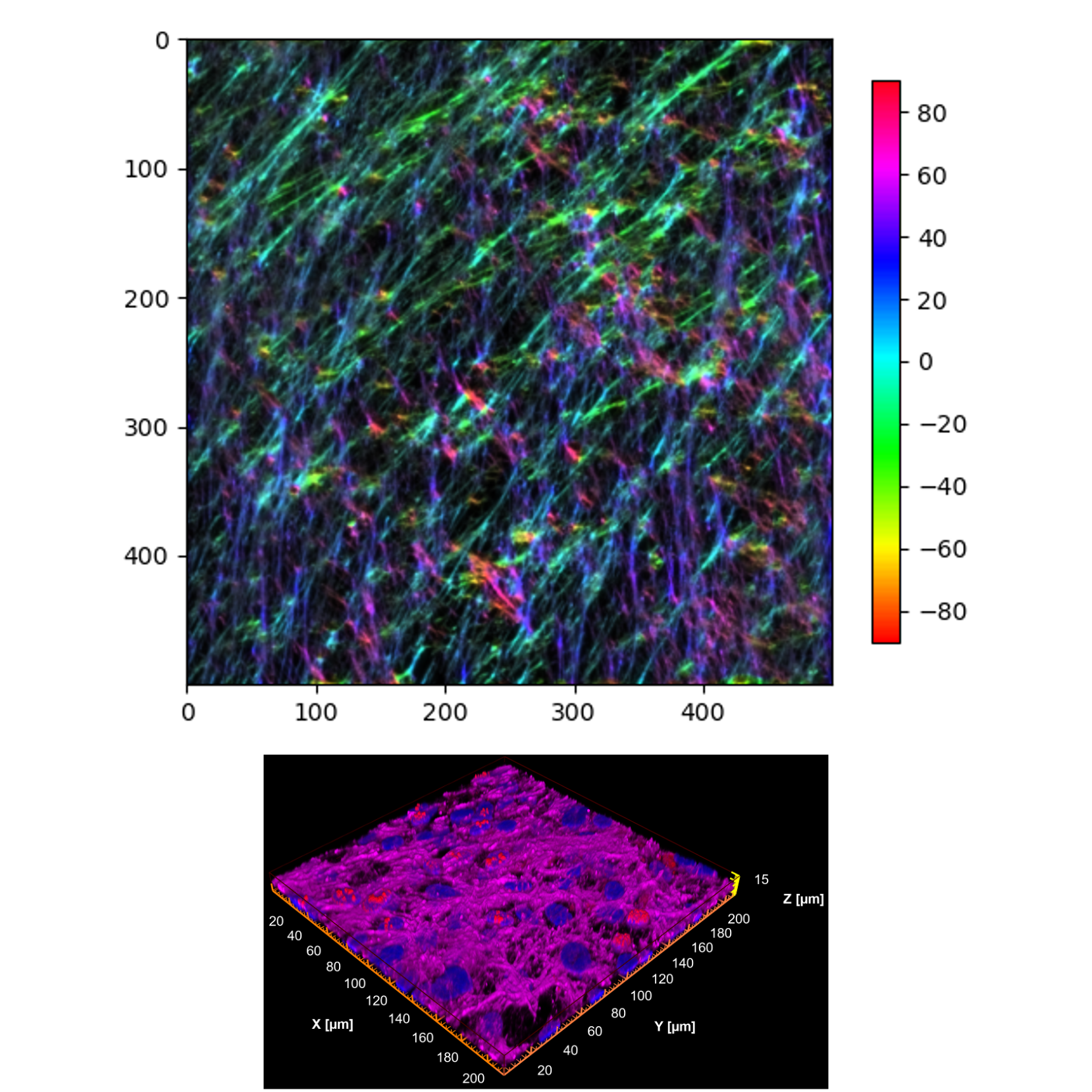
Within Images, a nested folder named normalized_images holds hue-normalized PNG outputs with the suffix _oj_analysis_normalized.png. These images re-map the OrientationJ hue space so that the modal fiber direction is centered (predominant fibers - cian); the embedded colorbar reflects deviation from the dominant direction in degrees (−90 to +90).
Example of FileName_oj_analysis_normalized.png
Use these normalized renders for consistent, cross-sample visual comparisons.
File naming follows the original base name of each input image. For example, an input experiment1.nd2 produces experiment1_processed.tif in the results root, experiment1_oj_distribution.csv in Excel, experiment1_oj_analysis.tif in Images, and experiment1_oj_analysis_normalized.png in Images/normalized_images. The processed analytics table appears as experiment1_oj_distribution_processed_<timestamp>.xlsx in Analysis, while the cohort roll-up is stored as Alignment_Summary_<timestamp>.xlsx.
Each input folder is processed independently and therefore contains its own Alignment_assay_results_angle_<ANGLE>_<TIMESTAMP> directory with the same internal structure. Console logs are printed during execution.
Expected result
Alignment_Summary.csv
| File_Name | Number_of_Z_Stacks | Z_Stack_Type | Percentage_Aligned_within_15° | Orientation_Mode | |
| Treatment_A.md2 | 32 | slices | 85.1376 | aligned | |
| Treatment_B.md2 | 24 | slices | 94.0664 | aligned |
Structure of result table for original fiber orientation assay. classified as aligned if ≥ 55%, else disorganized. Angle mode (15 degree can be changed by user).
UMA-tools: Fibronectin fibers alignment distribution by OrientationJ using python library
This module provides an alternative, Python-based implementation of fibronectin alignment analysis that replaces the OrientationJ plugin workflow. Because the algorithms and parameterizations differ, absolute values may vary from the OrientationJ outputs; however, the qualitative trends and sample-to-sample rankings are expected to remain consistent. For methodological continuity, we recommend running both approaches on a shared benchmark dataset, comparing key summary metrics (e.g., alignment percentage within a defined angle), and documenting any systematic offsets before adopting this script as a primary or cross-platform solution.
The script can be run on Windows (via WSL), Linux, and macOS. We recommend using Visual Studio Code for a consistent experience. Before execution, ensure that your dataset is prepared as folder-based confocal Z-stacks, all dependencies are installed, the project environment is created and activated, and the JSON configuration file points to the correct input locations.
Run the main analysis script:
python UMA-tools/code/alignment_analysis.py -i UMA-tools/input_paths.json
To change the default angle (15°), add the -a parameter (e.g., 5, 10):
python UMA-tools/code/alignment_analysis.py -i UMA-tools/input_paths.json -a 10
Follow instructions:
- Enter fibronectin channel index (starting from 1): you can find the channel number by opening the image in the FIJI GUI
- Do you want to start processing? (y/n):
OUTPUT DATA:
After a successful run, each input folder contains a new results directory named Alignment_assay_results_angle_<ANGLE>_<YYYYMMDD_HHMMSS>. This directory is the root for all outputs from that folder.
- The script writes 2D, max-projected fibronectin images directly into this root as <basename>_processed.tif; these are the resized grayscale projections used for downstream analysis. A log file (log.log) is also created in the same directory, recording key steps and messages.
Two subfolders are created: Tables and Images:
- The Tables folder stores per-image orientation distributions generated by the Python pipeline as CSV files named <basename>_orientation_distribution.csv.
- The Images folder stores visualization outputs: <basename>_orientation_composition.png shows the hue-encoded orientation map with a colorbar in degrees, and a nested Images/normalized_images folder contains <basename>_normalized_orientation.png, where hues are shifted so the modal fiber direction is centered; the colorbar indicates deviation from the dominant direction in degrees.
- An Analysis subfolder is created for post-processing results. For every CSV in Tables, the script writes a processed version named <basename>_orientation_distribution_processed.csv that includes angles normalized to the mode, corrected angle bounds, rank indices, and percentage contributions per bin. The script also compiles a study-level summary file named Alignment_Summary.csv, listing each image, the number and type of Z stacks recorded during projection, the percentage of fibers aligned within the specified angle window, and the final qualitative label (aligned or disorganized).
File naming preserves the original base name of each source image, so a file like sample01.nd2 yields sample01_processed.tif in the results root, sample01_orientation_distribution.csv in Tables, sample01_orientation_composition.png in Images, sample01_normalized_orientation.png in Images/normalized_images, sample01_orientation_distribution_processed.csv in Analysis, and a consolidated Alignment_Summary.csv summarizing all processed images for that input folder.
Expected result
Example of <filename>_processed.tif
2. Tables/<image>_orientation_distribution.csv
- Table of orientation angles and their corresponding occurrence frequencies.
- Contains two columns:
- occ_value : how often that angle appears in the image
- ori_angle: orientation angle in degrees (range: -90 to +90)
| ori_angle | occ_value | |
| -89.5 | 40541 | |
| -88.5 | 37202.25 | |
| -87.5 | 11174.25 | |
| -86.5 | 15646.75 | |
| -85.5 | 24988.5 | |
| -84.5 | 9602.25 | |
| -83.5 | 23665.5 | |
| cont... | cont... |
Example of the first 8 rows of
<image>_processed_orientation_distribution.csv
3. Images/<image>_orientation_composition.png
- RGB visualization where:
- Hue encodes orientation angle
- Saturation encodes coherence (directionality)
- Brightness encodes original image intensity
- Includes a colorbar showing angle scale from -90 to +90 degrees
4. Images/normalized_images/<image>_processed_normalized_orientation.png
- RGB visualization where:
- Hue encodes orientation angle
- Saturation encodes coherence (directionality)
- Brightness encodes original image intensity
- Includes a colorbar showing angle scale from -90 to +90 degrees relative to the dominant (cian) direction of the sample's fibronectin.
5. Analysis / <image>_orientation_distribution_processed.csv
Processed table with normalized angles and additional computed fields:
- ori_angle: orientation angle in degrees (range: -90 to +90)
- occ_value: how often that angle appears in the image
- angles_normalized_to_angle_of_MOV : angle shifted to the peak direction
- corrected_angles : wrapped angles into [-90°, +90°] range
- rank_of_angle_occ_value : rank order of angles by frequency
- perc_occvalue2sum_of_occvalue : angle frequency as a percentage
| ori_angle | occ_value | angles_normalized_to_angle_of_MOV | corrected_angles | rank_of_angle_occ_value | perc_occvalue2sum_of_occvalue | |
| -78.5 | 4331.25 | -90 | -90 | 1 | 0.001702338 | |
| -77.5 | 20457.25 | -89 | -89 | 2 | 0.00804044 | |
| -76.5 | 10260.25 | -88 | -88 | 3 | 0.00403265 | |
| -75.5 | 6347 | -87 | -87 | 4 | 0.002494601 | |
| -74.5 | 8573.5 | -86 | -86 | 5 | 0.003369696 | |
| -73.5 | 10525.5 | -85 | -85 | 6 | 0.004136902 | |
| cont... | cont... | cont... | cont... | cont... | cont... |
6. Analysis/Alignment_Summary.csv
- One-row summary per image.
- Contains:
- File name
- Number of Z-stacks
- Z-stack type
- Percentage of fibers aligned within the specified angle
- Orientation classification (aligned if ≥55% of fibers fall within the angle, otherwise disorganized)
| File_Name | Number_of_Z_Stacks | Z_Stack_Type | Percentage_Fibers_Aligned_Within_15_Degree | Orientation_Mode | |
| filename_processed_orientation_distribution.csv | 58 | slices | 66.07352435 | aligned |
6. log.log
- Log file for tracking errors, warnings, and progress during processing.
UMA-tools: fibroblast/ECM unit thickness assay based on fibrinectin staining
This script estimates ECM thickness from the fibronectin signal in multilayered fibroblast/ECM functional units. It is intended as a convenient, rapid QC-oriented assay to screen images, assess matrix quality for downstream analyses, and probe condition-dependent effects.
This is only one of several valid approaches to thickness measurement, and users may choose alternative methods as needed. Meaningful comparisons require a control group and/or an external gold standard analyzed by another method to anchor the measurements and enable cross-method validation.
Note
MACRO for ImageJ:
This workflow mirrors the automated Python pipeline and can be executed directly in ImageJ/Fiji to verify or reproduce individual steps. First, the image is opened with Bio-Formats as a hyperstack. The selected channel is resliced to generate an XZ view suitable for thickness mapping, then collapsed with a maximum-intensity Z-projection to obtain a 2D representation of the fibronectin layer. A sequence of denoising and enhancement filters follows: a Maximum filter (radius 2) to connect thin fibers, Gaussian Blur (σ = 2, scaled) to reduce high-frequency noise, and rolling-ball background subtraction (radius 50, sliding). The image is then thresholded with Otsu (dark) and converted to a binary mask with a black background, producing a fiber-only segmentation.
The Local Thickness plugin is run in masked, calibrated, silent mode to compute a per-pixel thickness map constrained to the segmented fibers and expressed in calibrated units when available. Measurement settings are configured to report area, standard deviation, minimum, and median, and a single call to Measure records these statistics to the Results table. In the Python-driven analysis described in this section, these same operations are orchestrated programmatically for batch processing; however, you can replicate or troubleshoot the procedure manually in ImageJ using the macro commands shown below.
Command
Macro for thickness assay for FIJI
Note: the first line requires an individual file input. If you want to analyze a batch of files in a folder, select the first file in the folder.
Run the main analysis script:
python UMA-tools/code/thickness_analysis.py -i UMA-tools/input_paths.json
Follow instructions:
- Enter 1 for .nd2 or 2 for .tiff:
- Enter the number of channels in the files: you can find the channel number by opening the image in the FIJI GUI
- Enter the channel number (1-3) representing fibronectin:
- Do you want to start processing? (y/n):
OUTPUT DATA:
After each run, every input folder gains a results directory named Thickness_assay_results_<YYYYMMDD_HHMMSS>. Inside, the script saves a log file (log.log) capturing processing steps and any warnings, plus one mask image and one thickness image per source file. The mask is written as Mask_<original_name>.tif and represents the binarized, max-projected fibronectin channel used to drive Local Thickness. The corresponding Local Thickness output is saved as Local_Thickness_<original_name>.tif, which contains the per-pixel thickness map produced by the plugin after reslice, projection, filtering, background subtraction, and thresholding.
A tabular summary for the folder is compiled into Thickness_Summary.csv, with one row per processed image reporting Area, StdDev, Min, Max, and Median. Units for thickness metrics (and Area) follow the image calibration present in the original files; if no spatial calibration is embedded, values are in pixels (and pixel-squared for Area). File base names are preserved, so a file like sample01.nd2 yields Mask_sample01.nd2.tif, Local_Thickness_sample01.nd2.tif, and a corresponding row in Thickness_Summary.csv. Each input folder is handled independently and therefore contains its own timestamped results directory with the same internal structure.
Expected result
Example of fibronectin channel in <filename>.nd2
1. Mask_<filename>.tif
A binary mask created by applying filtering and thresholding to the projected fibronectin channel. This serves as the input for the local thickness measurement.
Example of mask_<filename>.tif
2. Local_Thickness_<filename>.tif
The output image generated by the Local Thickness plugin. Each pixel value in this image corresponds to the estimated local thickness of the fibronectin matrix at that location.
Example of Local_Thickness_<filename>.tif
3. Thickness_Summary.csv
A summary table that aggregates quantitative measurements for all processed images in the folder. Each row corresponds to an image and includes the following columns:
| File_Name | Area | StdDev | Min | Max | Median | |
| example_001.nd2 | 1089.248 | 8.427518 | 1 | 16.5 | 8 | |
| example_002.nd2 | 1148.772 | 8.674721 | 1 | 8 | 7 |
Structure of result table for thickness assay (Thickness_Summary.csv). File_Name: Original filename of the image. Area: Total area (in calibrated units²) of the mask used for analysis. StdDev: Standard deviation in local thickness. Min: Minimum local thickness. Max: Maximum local thickness. Median: Mean local thickness across the mask.
UMA-tools: Nuclei counts and layers prediction
Confocal datasets are hindered by two practical constraints: the time required for manual slice-by-slice inspection of Z-stacks and background signal from nuclear dyes (e.g., DAPI) that makes nuclei counting difficult when using standard FIJI/ImageJ thresholding and particle analysis.
To address these challenges, the workflow employs an AI-based StarDist model for 3D segmentation of nuclei, wrapped in a Python pipeline that standardizes preprocessing, segmentation, and quantitative readouts. Processing is organized into three scripts:
Script 1 extracts the nuclei channel and applies 3D denoising to stabilize downstream segmentation; Script 2 performs StarDist3D segmentation and generates QC overlays;
Script 3 quantifies per-nucleus features and predicts the number of nuclear layers, producing both per-image and batch summaries. This structure provides a relatively rapid and reproducible approach for counting nuclei and estimating layer number in multilayered fibroblast/ECM units.
Before running the scripts, edit UMA-tools/nuclei_layers.json - at minimum, provide the path to your StarDist model, the paths to the raw .nd2/.tiff files, the nuclei channel number, and other parameters marked in bold:
{
"folder_paths": [
"path1",
"path2"
],
"nuclei_channel": 1 (index of the nuclei channel (starting from 1)),
"gaussian_sigma": 4.0 (Gaussian Blur 3D sigma for denoising),
"mean_radius": 3 (Mean 3D filter radius for smoothing),
"z_scale_factor": 32 multiplier applied to the Z axis for clustering,
"n_tiles": [2, 4, 4] (StarDist tiling in Z,Y,X (e.g., [z, y, x]) to handle large volumes),
"downscale_factor": 2 (optional downscaling of images before processing (integer)),
"model_path": "path" (filesystem path to the StarDist 3D model to use)
}
Note
"path_to_stardist_model" explanation: If this path is not provided, the script loads the default StarDist DEMO model (https://github.com/stardist/stardist); however, using a lab-specific model trained on your imaging conditions is strongly recommended for accurate results.
Models for the protocol to analyse fibronectin/ECM units are stored in UMA-tools/stardist_models_nuclei_layers. These differ by training dataset resolution (512 or 1024) and by the objective used during acquisition (60× or 40×). Choose the model that matches your data (voxel size, image resolution, objective) or train a new one on your own dataset.
Specify the full absolute path to the desired model in the configuration so the script can load it at runtime. If model performance is suboptimal, switch to a closer-matching model or retrain on representative images, then re-run the pipeline and verify using the QC overlays.
Run script 1:
python UMA-tools/code/1_nla_fiji_channel_extraction.py -i UMA-tools/nuclei_layers.json
Expected result
After completion, each dataset folder listed in the JSON is reset to a clean layout and contains four subdirectories: processed, masks, analysis, and clustering alongside a run log named nuclei_analysis1.log.
This first-step module populates only the processed folder: for every readable .nd2/.tif/.tiff input, it writes a channel-extracted 3D stack as <original_basename>_nuclei.tif, produced by duplicating the user-specified nuclei channel, converting to 8-bit, and applying Gaussian Blur 3D followed by Mean 3D (set up in UMA-tools/nuclei_layers.json file). File base names are preserved for traceability, and processing occurs in sorted order. The masks, analysis, and clustering folders are created empty here to standardize downstream steps. The per-folder nuclei_analysis1.log records all actions, including saved outputs and any files skipped due to unreadability or out-of-range channel indices.
Run script 2:
python UMA-tools/code/2_nla_stardist_prediction.py -i UMA-tools/nuclei_layers.json
Note
The program uses either the standard StarDist model or a model located in UMA-tools/stardist_models_nuclei_layers. If nuclear masks are displayed incorrectly, adjust the threshold parameters in the model’s thresholds.json specifically the Probability/Score Threshold and the Overlap Threshold. For details on these parameters, see https://imagej.net/plugins/stardist and https://github.com/stardist/stardist.
Expected result
After this second step, each dataset folder gains new outputs in the masks subdirectory and a run log named nuclei_analysis2.log at the folder root. For every preprocessed stack found in processed, the script writes an labeled nuclei mask as <basename>_mask.tif , where pixel value encode individual nuclei IDs across the full Z range. Alongside each mask, a quick-look quality-control image <basename>_QC.png is produced, showing the mid-Z slice with a semi-transparent label overlay and a title reporting the number of detected nuclei.
The log records the StarDist model used (custom model_path or the built-in 3D_demo), the tiling configuration n_tiles, per-image shapes before prediction, and the nuclei count written to each mask, as well as any exceptions raised during processing. The script preserves the original base names from processed, ensuring traceability between the input stacks and their corresponding masks and QC images.
Run script 3:
python UMA-tools/code/3_nla_fiji_calculation.py -i UMA-tools/nuclei_layers.json
After the third step, each dataset folder contains new outputs in analysis and clustering along with a run log nuclei_analysis3.log at the folder root. For every nuclei mask in masks, the script writes a per-image quantification table to analysis as <basename>_analysis.csv with one row per nucleus, including nucleus_id, vol_vox (voxel count), centroid coordinates (x, y, z), and equivalent diameter in pixels; a QC figure <basename>_3D_QC.png is also saved showing colorized XY, XZ, and YZ maximum-intensity projections of instance labels with centroid overlays. Using these per-image CSVs, the script performs depth-aware clustering and saves to clustering two outputs per image: <basename>_clusters.csv, which appends cluster_xz and cluster_yz labels for each nucleus and records all nuclei including those labeled −1 as unclustered, and <basename>_cluster_4proj.png, a four-panel figure displaying XZ and YZ HDBSCAN clusters and the corresponding XY projections colored by each clustering. A folder-level summary clustering_summary.csv is written to clustering, aggregating image-level statistics such as Total_Nuclei, counts of XZ/YZ clusters, unclustered nuclei, and per-cluster sizes; if multiple dataset folders are listed, a consolidated summary is additionally saved in the clustering directory of the first folder. All filenames preserve the original base names for traceability, spatial units reflect the upstream calibration (otherwise pixels), and visualization axes use the original coordinate frame with the configured z_scale_factor applied internally for clustering only.
Expected result
All directories specified below are automatically generated by the script within the folder containing your unprocessed 3D images.
Clustering Summary .csv
A summary .csv file denoting the number of predicted nuclei in predicted each layer of each image is generated within the input folder like the example below:
| A | B | C | D | E | F | |
| Image | Layer 1 | Layer 2 | Layer 3 | Layer 4 | Unclustered | |
| no rad no gem cs2_002_nuclei_resized | 17 | 15 | 10 | 0 | 18 | |
| PLDR+ gem cs2_004_nuclei_resized | 0 | 0 | 0 | 0 | 24 | |
| uma-images-test_nuclei_resized | 0 | 0 | 0 | 0 | 24 | |
| no rad no gem cs2_001_nuclei_resized | 17 | 10 | 24 | 38 | 15 |
Summary .csv file example
Analysis/
.csv File: For each mask corresponding to a 3D image, the dimensions and centroid coordinates of all predicted nuclei are extracted and saved in a .csv file like the example below:
| nucleus_id | volume_voxels | z_pos | y_pos | x_pos | bbox-0 | bbox-1 | bbox-2 | bbox-3 | bbox-4 | bbox-5 | solidity | diameter_um | volume_um3 | |
| 1 | 122090 | 13.763133753788189 | 181.03407322467032 | 425.87568187402735 | 4 | 131 | 372 | 25 | 230 | 478 | 0.9254149927992117 | 61.54987243057981 | 366.27000000000004 | |
| 2 | 103930 | 11.508130472433368 | 458.72164918695273 | 487.7680169344751 | 2 | 413 | 436 | 24 | 502 | 539 | 0.9174368616650336 | 58.332971710466346 | 311.7900000000001 | |
| 3 | 109269 | 13.865625200194017 | 228.32991973935884 | 611.285635 | 5 | 188 | 551 | 25 | 267 | 669 | 0.92673887 | 59.31521588563253 | 327.8070000000001 | |
| 4 | 79637 | 16.166116252495698 | 337.57508444567225 | 388.8243655587227 | 6 | 284 | 358 | 27 | 392 | 421 | 0.9223971182691083 | 53.37920356576035 | 238.91100000000003 |
Per-image CSV generated from each 3D mask
Quality Control Plots: For each mask corresponding to a 3D image, a quality control plot in .png format containing the following components is generated:
- A maximum intensity XY projection of nuclei predicted by your StarDist model, indicating the total
- XZ and YZ projections of nuclei predicted by your StarDist model
Clustering/
For each input image, an XZ plot in .png format displaying predicted nuclei centroids organized into clusters (and unclustered nuclei) is generated.
Masks/
The 'masks' directory should contain 3D masks in .tif format showing StarDist-predicted nuclei and corresponding quality control images that show the middle slice of a processed 3D image next to the corresponding slide of its mask.
3D TIFF masks of StarDist-segmented nuclei with corresponding QC images: the mid-Z slice of the preprocessed volume shown alongside the matching slice of its label mask.
Processed/
The 'processed' directory should contain processed versions of your .nd2 images saved under the same filename in .tif format. In this case, processing means that Gaussian Blur 3D and Mean 3D filters have been applied and your nuclei-containing channel has been isolated.
Schematic of nuclei-channel Z-stack preprocessing: Gaussian Blur 3D followed by Mean 3D filtering prior to segmentation.
Note
This script clusters nuclei centers based on their spatial density using the HDBSCAN algorithm, using the default excess of mass (EOM method). EOM works by examining the density of clusters under varying conditions and favors clusters that persistently remain dense. During clustering, the Z coordinates of nuclei centers are scaled according to the user-specified Z scale factor to account for anisotropy between the XY and Z resolutions of an image. In other words, this value helps maintain spatial accuracy during clustering.
2. CLUSTERING PARAMETERS
Parameters affecting the HBDSCAN clustering algorithm, with the exception of z-scale factor can be modified within code 3_nla_fiji_calculation.py. Detailed explanations of each parameter, as well as the expected effects of changing them are available within the scikit-learn library documentation.
HDBSCAN(
min_cluster_size=actual_min_cluster_size,
min_samples=actual_min_samples,
cluster_selection_epsilon=epsilon,
n_jobs=-1
).fit(xz_coords)
csv_path: Path,
out_dir: Path,
z_scale: int = 10,
summary: list = None,
*,
trim_method: str = "MAD",
k: float | tuple = 2.5,
min_cluster_size: int = 5,
min_samples: int = 3,
epsilon: float = 4.0,
min_nuclei: int = 10,
normalize: bool = True,
point_size: int = 60) -> dict:
FIA-tools: foci imaging assay
FIA-tools is a modular (four consecutive scripts) foci imaging assay designed to quantify nuclear foci and related markers in multilayered fibroblast/ECM functional units. It can also analyze 2D TIFF images of nuclei, provided they are compatible with the standard StarDist (https://stardist.net) model (2D_versatile_fluo) - i.e., fluorescent nuclear signal, adequate contrast, and an appropriate spatial scale. The workflow operates on 2D XY projections of nuclei, applies the standard StarDist model (2D_versatile_fluo) to segment nuclei reliably in the presence of potential background and debris, and then performs foci detection, optional multi-channel colocalization, and quantitative readouts using FIJI/ImageJ operations. The pipeline is organized as several scripts that prepare images, segment nuclei, generate foci masks, and compile per-nucleus metrics, enabling batch processing across multiple folders and datasets while preserving transparent intermediate outputs and logs.
Compared with a standard GUI-centric solution such as CellProfiler (https://cellprofiler.org), FIA-tools offers fine-grained, Python-first control, direct integration with StarDist and FIJI/ImageJ, explicit metadata handling, and easy extensibility for custom analyses or lab-specific conventions. These features can improve reproducibility, facilitate troubleshooting, and simplify cross-platform use when proprietary formats (e.g., .nd2 and TIFF/TIF) and FIJI macros are part of the workflow. At the same time, CellProfiler may be preferable when a point-and-click interface, mature module library, turn-key pipelines, and centralized project management are priorities. FIA-tools requires limited user input at defined stages, a multi-script execution model, and familiarity with VS Code and environments, which can introduce additional setup time relative to an end-to-end CellProfiler pipeline. In practice, both approaches are complementary: use FIA-tools when you need StarDist-driven segmentation, ImageJ interoperability, and programmable control; use CellProfiler for rapid prototyping and GUI-based batch analyses.
The script can be run on Windows (via WSL), Linux, and macOS. We recommend using Visual Studio Code for a consistent experience. Before execution, ensure that your dataset is prepared as folder-based confocal Z-stacks, all dependencies are installed, the project environment is created and activated, and the JSON configuration file points to the correct input locations.
Run the first script of FIA-tools:
python FIA-tools/code/1_select_channels.py -i FIA-tools/input_paths.json
- Launch check and input file selection Start analyzing files in the specified folders? (yes/no): If yes, the program validates that the folders are listed in the JSON file and inspects their contents.
- Select input file type:
- ND2 files (multi-channel Z-stacks)
- Multi-channel TIFF files with Z-stacks
- 2D multi-channel TIFF files (already projections) Enter choice (1-3):
- Define channels Enter the channel number for nuclei staining (starting from 1): • Determine the nuclei channel by opening a representative image in FIJI and viewing split channels. How many foci channels do you want to process?: • Enter the count of foci channels to analyze (e.g., 1, 2, or more). Enter the channel number for Foci 1 (starting from 1): Enter the channel number for Foci 2 (starting from 1): • Repeat as needed for each foci channel.
Note
Lines 12–18 (1_select_channels.py) configure the Java heap size at 16 GB to improve computational throughput. On systems with less available RAM, this value should be reduced (e.g., to 4 GB) to prevent memory overcommitment and ensure stable execution.
Note
For FIA-tools to run, the file FIA-tools/input_paths.json must list the data directories. Use absolute paths to the folders that contain your images (e.g., .nd2 or .tif/.tiff files).
The output of this program is a foci_assay folder created in each image folder listed in the JSON file. Inside, two subfolders will be generated:
- Nuclei folder
- Foci folder
Each subfolder will contain the extracted image channels that will be used for further analysis. Additionally, in the foci_assay folder, there will be a image_metadata.txt where information about the pixel size in micrometers from the original files is saved.
Expected result
Nuclei/
<image>_nuclei_projection.tif
For .nd2 files: Max-intensity Z-projection of the specified nuclei channel.
For .tif/.tiff: Extracted single 2D channel image.
All images are resized to 1024×1024 pixels and converted to 8-bit TIFF.
Example of <image>_nuclei_projection.tif
Foci/Foci_<i>_Channel_<N>/
<image>_foci_projection.tif:
For .nd2: Standard deviation (SD) Z-projection of the specified foci channel.
For .tif/.tiff: Extracted 2D channel image.
Each image is resized to 1024×1024 pixels and converted to 8-bit TIFF.
Example of <image>_foci_projection.tif
Metadata and logs:
image_metadata.txt:
A plain text file listing image-specific metadata for all processed files:
For each image:
- Pixel dimensions (width, height, depth)
- Calibration units (e.g., µm)
- Number of channels, Z-slices, and time frames
1_log.txt:
- Contains all warning and error messages generated during processing
- Includes info about skipped files, invalid channel requests, or failed image reads
Run second script:
python FIA-tools/code/2_nuclei_mask_generation.py -i FIA-tools/input_paths.json -p 500
This value (e.g., 500) sets the nucleus size threshold - any detected objects smaller than this will be considered noise and excluded.
Expected result
This script performs two main steps:
- Nuclei detection using a deep learning model (StarDist2D) and saves labeled masks.
- ImageJ-based mask processing including thresholding, watershed, and particle analysis.
Each input folder listed in the JSON file (used previously in foci_assay/) results in the creation of two new result folders, each with its own log and image output.
<TIMESTAMP>:Date-time string in format YYYYMMDD_HHMMSS indicating when processing occurred.
<image>: The base name of the image file being processed.
Step 1 – StarDist Nuclei Detection
Nuclei_StarDist_mask_processed_<timestamp>/
*_StarDist_processed.tif:
- 16-bit labeled instance masks of nuclei predicted by StarDist2D model (2d_versatile_flux).
- Each label corresponds to a unique nucleus.
Example of *_StarDist_processed.tif
2_log.txt:
- Log file for errors and warnings encountered during the StarDist processing.
- Includes file type validation, model prediction issues, or unsupported formats.
Step 2 – ImageJ Mask Post-processing
Final_Nuclei_Mask_<timestamp>/
- Binary masks post-processed in ImageJ:
Thresholded
Converted to binary mask
Watershed applied
Particles filtered based on size (default ≥ 2500 px)
Output is a final mask used for quantification of foci overlap, etc.
Example of Final Nuclei Mask
- nuclei_log.txt:
Captures any image opening errors, unsupported file types, or issues during particle analysis.
Run third script:
python FIA-tools/code/3_foci_mask_generation.py -i FIA-tools/input_paths.json -f 50
The third script is used to create black-and-white masks for Foci. Since the background intensity can vary for each channel, this program is run separately for each channel. For example, you specify the -f parameter, which sets the background intensity threshold—any signal below this value will be discarded.
Follow instruction:
- Subfolders found across all Foci folders:
1) Foci_1_Channel_1
..
...
- Select subfolder to analyze (enter a number): 2
- You selected 'Foci_2_Channel_2'. Proceed? (yes/no):
Expected result
This script filters foci channels using a user-defined intensity threshold, applies binarization, watershed segmentation, and generates per-image binary masks. The operation is performed on a user-specified subfolder within the Foci/ directory for all valid input folders.
Folder Layout per Input Directory
For each <input_folder> (from JSON), this script reads from the foci_assay/ structure and outputs new results in the following hierarchy:
<timestamp>: A unique datetime stamp in YYYYMMDD_HHMMSS format indicating when processing begun.
<image>The original filename without extension.
Output Description:
1. Foci_Masks/<chosen_subfolder>_<timestamp>/
This is the main output folder containing processed data from the selected foci channel.
- processed_<imege>.tif:
Binary mask created from the input image using:
intensity thresholding (default ≥150)
watershed segmentation
particle analysis (Analyze Particles... in ImageJ)
This file highlights individual foci regions and is suitable for downstream quantification and colocalization.
Example of processed_<image>.tif
- foci_log.txt
Log file capturing any image reading errors, missing metadata, or unsupported files.
- image_metadata.txt (read-only)
Used to retrieve pixel calibration (µm per pixel) from previously generated metadata (Step 1).
If unavailable for a file, the script falls back to default values (0.207 µm/pixel).
- 3_val_log.txt
Per-input-folder log generated during validation.
Reports missing foci_assay/, empty folders, or incorrect file types.
Run script 4:
python FIA-tools/code/4_foci_quantification.py -i FIA-tools/input_paths.json
Follow instructions:
- Start processing? (yes/no):
- Do you want to perform colocalization analysis? (yes/no):
Expected result
Output Structure: Nuclei–Foci Quantification and Colocalization Summary (Step 4)
This script performs quantitative analysis of foci signals within previously segmented nuclei using masks from prior steps. It generates:
- Summary statistics per nucleus
- Optional colocalization between foci channels
- Final labeled images
- Colocalized binary masks
- A consolidated CSV file for downstream statistical analysis
<TIMESTAMP>:Date-time string in format YYYYMMDD_HHMMSS indicating when processing occurred.
<image>: Original image key, cleaned from filename
<channels>: Amount of intersected channel names (e.g.,
Foci_1_Channel_1+Foci_2_Channel_2)
Output Content Description:
1. all_results_with_coloc_universal.csv
A master CSV table with one row per nucleus, including:
- Nucleus ID and image identifier (Image Key, Nucleus)
- Nucleus area in pixels and micron²
- For each foci channel:
Foci count
Total foci area in pixels and micron²
Relative foci coverage (% of nucleus)
- If colocalization is enabled:
Same statistics for each subset of overlapping foci channels (2-way, 3-way, etc.)
2.*_labeled_nuclei.png
- Visual representation of each nuclei mask with label numbers overlaid
- Used for manual validation and visual tracing of nuclei IDs used in the CSV
3. intersection_<image_key>_<channel_combo>.tif
- Colocalized binary masks for all foci channels in the specified combination
- Format: black objects (labelled foci), white background
- Useful for confirming overlap visually or performing additional analyses
Note: this example only has 1 foci channel. If multiple foci channels are present, the image represents the overlay of all selected foci masks.
4. 4_log.log
Comprehensive logging of the run.
Protocol references
The protocol for 3-D fibroblastic units production was based on the following protocols:
1. Franco-Barraza J, Beacham DA, Amatangelo MD, Cukierman E. Preparation of Extracellular Matrices Produced by Cultured and Primary Fibroblasts. Curr Protoc Cell Biol. 2016 Jun 1;71:10.9.1-10.9.34. doi: 10.1002/cpcb.2. PMID: 27245425; PMCID: PMC5058441. https://currentprotocols.onlinelibrary.wiley.com/doi/10.1002/cpcb.2
2. Franco-Barraza J, Raghavan KS, Luong T, Cukierman E. Engineering clinically-relevant human fibroblastic cell-derived extracellular matrices. Methods Cell Biol. 2020;156:109-160. https://doi.org/10.1016/bs.mcb.2019.11.014 Epub 2020 Jan 21. PMID: 32222216; PMCID: PMC7298733.
The following software programs were used to develop the protocol for analyzing the characteristics of the 3-D fibroblastic matrix:
Schneider, C. A., Rasband, W. S., & Eliceiri, K. W. (2012). NIH Image to ImageJ: 25 years of image analysis. Nature Methods, 9(7), 671–675.doi:10.1038/nmeth.2089
FIJI: https://fiji.sc Schindelin J, Arganda-Carreras I, Frise E, Kaynig V, Longair M, Pietzsch T, Preibisch S, Rueden C, Saalfeld S, Schmid B, Tinevez JY, White DJ, Hartenstein V, Eliceiri K, Tomancak P, Cardona A. Fiji: an open-source platform for biological-image analysis. Nat Methods. 2012 Jun 28;9(7):676-82. doi: 10.1038/nmeth.2019. PMID: 22743772; PMCID: PMC3855844.
StarDist:
1. Schmidt, U., Weigert, M., Broaddus, C., Myers, G. (2018). Cell Detection with Star-Convex Polygons. In: Frangi, A., Schnabel, J., Davatzikos, C., Alberola-López, C., Fichtinger, G. (eds) Medical Image Computing and Computer Assisted Intervention – MICCAI 2018. MICCAI 2018. Lecture Notes in Computer Science(), vol 11071. Springer, Cham. https://doi.org/10.1007/978-3-030-00934-2_30
2. Weigert, Martin, et al. "Star-convex polyhedra for 3D object detection and segmentation in microscopy." Proceedings of the IEEE/CVF winter conference on applications of computer vision. 2020. doi:10.1109/WACV45572.2020.9093435 https://openaccess.thecvf.com/content_WACV_2020/papers/Weigert_Star-convex_Polyhedra_for_3D_Object_Detection_and_Segmentation_in_Microscopy_WACV_2020_paper.pdf
3. Weigert, Martin, and Uwe Schmidt. "Nuclei instance segmentation and classification in histopathology images with stardist." 2022 IEEE International Symposium on Biomedical Imaging Challenges (ISBIC). IEEE, 2022. doi: 10.1109/ISBIC56247.2022.9854534 https://ieeexplore.ieee.org/abstract/document/9854534
1. Püspöki Z, Storath M, Sage D, Unser M. Transforms and Operators for Directional Bioimage Analysis: A Survey. Adv Anat Embryol Cell Biol. 2016;219:69-93. doi: 10.1007/978-3-319-28549-8_3. PMID: 27207363. https://bigwww.epfl.ch/publications/puespoeki1603.html
2. Rezakhaniha R, Agianniotis A, Schrauwen JT, Griffa A, Sage D, Bouten CV, van de Vosse FN, Unser M, Stergiopulos N. Experimental investigation of collagen waviness and orientation in the arterial adventitia using confocal laser scanning microscopy. Biomech Model Mechanobiol. 2012 Mar;11(3-4):461-73. doi: 10.1007/s10237-011-0325-z. Epub 2011 Jul 10. PMID: 21744269. https://bigwww.epfl.ch/publications/rezakhaniha1201.html
3. Fonck E, Feigl GG, Fasel J, Sage D, Unser M, Rüfenacht DA, Stergiopulos N. Effect of aging on elastin functionality in human cerebral arteries. Stroke. 2009 Jul;40(7):2552-6. doi: 10.1161/STROKEAHA.108.528091. Epub 2009 May 28. PMID: 19478233. https://bigwww.epfl.ch/publications/fonck0901.html
Skit-learn:
Pedregosa, Fabian, et al. "Scikit-learn: Machine learning in Python." the Journal of machine Learning research 12 (2011): 2825-2830.
Acknowledgements
We dedicate this work to Patricia Keely (a pioneer in ECM biology) and Neelima Shah (the most beautiful soul), whose inspiration continues to guide our studies.
This work was supported by the 5th AHEPA Family Cancer Research Foundation, the Pancreatic Cancer Cure Foundation, and the Community Foundation of New Jersey (Marina Zazanis). NIH grants: R01CA269660, U54CA272686, and equipment grant S10ODO23666. Additional funding was provided by DOD grant HT9425-23-1-0584, the ACS Wilmott Family Pancreatic Cancer Professorship RP-23-1070169-01-WRP, and the NIH/NCI Comprehensive Cancer Center Core Grant P30CA06927, supporting the Bio Sample Repository, Cell Culture, Imaging, Radiation, Biostatistics and Bioinformatics, and Histopathology (both branches).