Dec 16, 2025
Ensuring accurate co-registration measurement for quality control of Single Point Confocal Laser Scanning Microscopes - V1
- Aurelien Dauphin1,
- Maria Azevedo2,3,
- Aidan Boyce4,
- Fabrice Cordelières5,
- Herlinde De Keersmaecker6,
- Frank Eismann7,
- Orestis Faklaris8,
- Hans Fried9,
- David Grunwald10,
- Christian Kukat11,
- Pascal Lorentz12,
- Tobie Martens13,
- Ileana Micu14,
- Roland Nitschke15,
- John Oreopoulos4,
- Allister Pattison4,
- Alex Payne-Dwyer16,
- Vincent Schoonderwoert17,
- Christian Schulz18,
- Maria Smedh19,
- Sathya Srinivasan20,
- Nicolas Stifani21,
- Kees van der Oord22,
- Nicolaas van der Voort23,
- Marlies Verschuuren24,
- Luis-Francisco Acevedo-Hueso25,
- Judith Lacoste26
- 1Unite Genetique et Biologie du Développement U934, PICT-IBiSA, Institut Curie, INSERM, CNRS, PSL Research University, Paris, 75005, France;
- 2Advanced Light Microscopy Scientific Platform, i3S – Instituto de Investigação e Inovação em Saúde | Porto, Portugal;
- 3University of Porto;
- 4Oxford Instruments;
- 5Bordeaux Imaging Center;
- 6Ghent Light Microscopy CORE, Ghent University, Ottergemsesteenweg 460, 9000 Ghent, Belgium;
- 7Carl Zeiss Microscopy GmbH, Jena, Germany;
- 8MRI, Biocampus, University of Montpellier, CNRS, INSERM, Montpellier, France;
- 9CRFS – Light Microscope Facility, German Center for Neurodegenerative Diseases (DZNE);
- 10UMass Chan Medical School;
- 11FACS & Imaging Core Facility, Max Planck Institute for Biology of Ageing, Cologne, Germany;
- 12Department of Biomedicine, University of Basel, Switzerland;
- 13Cell Imaging Core, KU Leuven;
- 14Queen's University Belfast;
- 15Life Imaging Center and Signalling Research Centres CIBSS and BIOSS, University of Freiburg, Germany;
- 16Bioscience Technology Facility, University of York;
- 17SVI;
- 18Leica Microsystems CMS GmbH;
- 19University of Gothenburg;
- 20Oregon National Primate Research Center (ONPRC, OHSU West Campus);
- 21UdeM;
- 22Nikon Europe BV;
- 23Scientific Volume Imaging;
- 24Antwerp Centre for Advance Microscopy, University of Antwerp, Antwerp, Belgium.;
- 25Quantum Medical Diagnostics;
- 26MIA Cellavie Inc, PO Box 192, Stn Anjou, Montréal QC Canada, H1K 4G6
- Aurelien Dauphin: Co-first authorship;
- Maria Azevedo: Co-first authorship;
- QUAREP-LiMiTech. support email: [email protected]


Protocol Citation: Aurelien Dauphin, Maria Azevedo, Aidan Boyce, Fabrice Cordelières, Herlinde De Keersmaecker, Frank Eismann, Orestis Faklaris, Hans Fried, David Grunwald, Christian Kukat, Pascal Lorentz, Tobie Martens, Ileana Micu, Roland Nitschke, John Oreopoulos, Allister Pattison, Alex Payne-Dwyer, Vincent Schoonderwoert, Christian Schulz, Maria Smedh, Sathya Srinivasan, Nicolas Stifani, Kees van der Oord, Nicolaas van der Voort, Marlies Verschuuren, Luis-Francisco Acevedo-Hueso, Judith Lacoste 2025. Ensuring accurate co-registration measurement for quality control of Single Point Confocal Laser Scanning Microscopes - V1. protocols.io https://dx.doi.org/10.17504/protocols.io.q26g7yrj8gwz/v1
License: This is an open access protocol distributed under the terms of the Creative Commons Attribution License, which permits unrestricted use, distribution, and reproduction in any medium, provided the original author and source are credited
Protocol status: Working
We use this protocol and it's working
Created: September 16, 2022
Last Modified: December 16, 2025
Protocol Integer ID: 70131
Keywords: Co-registration, chromatic aberration, colour shift, fluorescence, quality control, QUAREP-LiMi, single point confocal laser scanning microscope, scanning confocal microscope, confocal microscope, axial displacements between fluorescence channel, spatial relationships in biological specimen, different wavelengths to the same focal position, chromatic aberration, fluorescence channel, v1 chromatic aberration, precise measurement of channel alignment, misalignment of optical component, objective lens imperfection, same focal position, biological specimen, precise measurement, channel alignment, refractive index variation, different wavelength
Disclaimer
This protocol collection was developed by members of WG4 "System chromatic aberration and co-registration" of the international consortium QUAREP-LiMi.
The Consortium for Quality Assessment and Reproducibility for Instruments and Images in Light Microscopy (QUAREP-LiMi), formed by the global community of practitioners, researchers, developers, service providers, funders, publishers, policy makers and industry related to the use of light microscopy, is committed to democratizing access to quantitative and reproducible light microscopy and the data generated by it.
This protocol collection has undergone the internal approval process of QUAREP-LiMi.
It is not the intention of this protocol collection to supplant the need for independent professional judgment, advice, diagnosis, or treatment. Any action taken or withheld on the basis of the information presented here is undertaken at the user's own risk. The user agrees that neither the company nor any of the authors, contributors, administrators, or other individuals associated with protocols.io or QUAREP-LiMi can be held liable for any injuries, damages, or losses incurred as a result of the user's use of the information contained in or linked to this protocol or any of our websites, applications, or services.
Abstract
Chromatic aberration is a major source of spatial inaccuracy in multi-color fluorescence microscopy, arising from the inability of optical systems to bring different wavelengths to the same focal position. These wavelength-dependent shifts can originate from objective lens imperfections, refractive index variations, or misalignment of optical components, and often manifest as lateral or axial displacements between fluorescence channels. Accurate co-registration of multi-color images is therefore essential for reliable interpretation of spatial relationships in biological specimens.
This protocol provides a streamlined and quantitative method to assess co-registration accuracy in laser-scanning confocal microscopes, following the principles of ISO 21073. While the ISO-recommended procedure is laborious and time-consuming, our approach offers a faster and more user-friendly alternative while remaining compatible with ISO specifications. Using 1-µm multi-color beads, the protocol enables precise measurement of channel alignment, facilitating routine performance monitoring and high-quality multi-color imaging.
Guidelines
This protocol focuses on measuring the co-registration accuracy of a single point confocal laser scanning microscope in x, y, and z for each fluorescence color available in this type of system. We define the following:
I. Sample Preparation.
II. Pre-requisites
III. Image Acquisition
IV. Data Analysis
Materials
Coverslips, grade #1.5H (170 ± 5 μm) thickness
Glass slides
Lens tissue
HCl 1M solution
Ethanol 100%
Distilled water
TetraSpeck Microspheres 0.200 μm in diameter: Thermo Fisher Scientific T7280 (https://www.thermofisher.com/order/catalog/product/T7280)
TetraSpeck Microspheres 1 μm in diameter: Thermo Fisher Scientific T7282 (https://www.thermofisher.com/order/catalog/product/T7282)
TetraSpeck Microspheres 4 μm in diameter: Thermo Fisher Scientific T7283 (https://www.thermofisher.com/order/catalog/product/T7283)
Mounting media, for example Prolong™ Gold, Thermo Fisher Scientific P39934
Protocol materials
Eco-SilPicodentCatalog #1300 6100
Tetraspeck™ microspheres, 1.0 µm, fluorescent blue/green/orange/dark redThermo ScientificCatalog #T7282
ProLong™ Gold Antifade MountantThermo FisherCatalog #P10144
ProLong™ Glass Antifade MountantThermo FisherCatalog #P36984
Troubleshooting
Problem
Objective Lens Chromatic Aberrations (the user can address)
Solution
Carefully check objective specifications to minimize color-dependent focal shifts. If possible, choose an apochromatic version of the objective to minimize chromatic aberrations.
Problem
Immersion Medium (Oil, Water, or Air) (the user can address)
Solution
Ensure that the medium is clear, has a correct refractive index and Abbe number, and is not out of date to avoid focal shifts, chromatic aberrations, or wavefront aberrations (like spherical aberration).
Problem
Clean objective (the user can address)
Solution
Clean your objective properly. Chromatic aberrations are often caused by dirt films on objectives.
Problem
Objective Collar Adjustment (if present) (the user can address)
Solution
Properly set for the correct coverslip thickness, medium, and temperature.
Problem
DIC Slider Positioning (the user can address)
Solution
Ensure the Differential Interference Contrast (DIC) slider is fully retracted or void when using the confocal mode to avoid beam path deviations.
Problem
Dichroic Mirrors and Beam Splitters (the user can address)
Solution
Ensure correct selection and consistent use across the different channel acquisitions to prevent spectral shifts between channels. Misaligned or mismatched dichroics can cause color registration errors.
Problem
Laser Beam Injection Alignment (need manufacturer assistance)
Solution
Verify precise beam alignment to prevent excitation shifts between channels.
Problem
Collimation of Laser Beams (need manufacturer assistance)
Solution
Ensure correct collimation for a consistent focal plane positioning across wavelengths. A 405 nm laser will often focus at a different position than blue, green, or red lasers. In most confocal scanning microscopes, the 405 nm laser path can be adjusted independently of the other lasers.
Problem
Galvanometric or Resonant Scanner Alignment (need manufacturer assistance)
Solution
Regularly calibrate scanners to prevent spatial drift between channels.
Before start
Chromatic aberration refers to possible artifacts caused by a wavelength-dependency of the imaging properties of any fixed optical beam path of the microscope system (as a result of optical design of the system, the manufacturing tolerances of the system, and the current state of alignment of the optical components).
Co-registration accuracy more generally refers to the ability of the system to co-localize dyes of different wavelengths during a particular experimental set-up. Depending on the experimental set-up and also the system architecture of the system to be tested, one might achieve different results. This could occur if the system architecture or experimental set-up force the system to use different beam paths for the experiment. The required switching of beam paths introduces an additional complication for the co-registration on top of the chromatic aberrations.
1) Prior knowledge of the microscope architecture is important in order to be able to set-up experiments with minimal mechanical switching movement for highest accuracy results. If the experiment requires mechanical switching of optical components, all available channel calibrations/adjustments should be performed successfully before any quality control measurement (for example pinhole alignment and beam splitters).
2) If the system allows for chromatic corrections (for example, different collimators for different excitation sources) or adjustments (software-based corrections), all corrections and adjustments have to be optimized prior to measurements and kept stable during measurements.
3) Objective lenses have different levels of correction for chromatic aberrations. Therefore they will differ in their performance with respect to spectral bandwidth within a given aberration budget and in their maximum aberration over a given spectral range. For example, objectives rated (according to ISO19012-2) as semiapochromats will typically have a smaller spectral bandwidth as well as larger residual aberrations within the visible wavelength range than apochromats. Semiapochromats are typically marked with a "FL" in their designation, like "Fluor", "FLUOTAR" or "Neofluar". Apochromats always contain "Apo" in their designation. Objectives which exceed the specifications of an apochromat are labelled as, for example,
"APO CS2", "Apo Lambda", "C-Apochromat" or "XAPO" to indicate an even higher level of chromatic correction.
4) The system and the specimen should also be in steady temperature state. To confirm a steady state is reached, recording the temperature during measurements close to the sample is recommended. Capturing this information in the metadata is recommended.
5) When using oil immersion objective, the immersion oil to be used should be clear to the eye, devoid of crystals, dirt etc.
In addition, be cautious to use only the specified oil for immersion objectives since small differences (in particular variations of the Abbe number) may influence the co-registration accuracy significantly. Capturing this information in the metadata is recommended (manufacturer, catalog number, lot number, refractive index, expiration date (if any) etc.).
Coverslip preparation
30m
Prepare coverslips, grade #1.5H (170 ± 5 μm) thickness (according to ISO8255-1). Immerse the coverslips in a 1M HCl solution and shake gently for 30 min at room temperature. 00:30:00 RT
30m
Rinse the coverslips twice with distilled water and immerse them in 100% ethanol for storage (up to several months).
Bead Selection
Beads with different diameters and fluorescent properties can be used for this protocol. Here, beads co-emitting blue (360/430 nm), green (505/515 nm), orange (560/580 nm), and dark red (660/680 nm) fluorescence with 1 µm diameter were used. The choice is based on tests (see Supplementary Information, Section 11).
Tetraspeck™ microspheres, 1.0 µm, fluorescent blue/green/orange/dark redThermo ScientificCatalog #T7282
Before starting
The bead size, fluorescence specifications, manufacturer, catalogue number, lot number, and expiration date (if any) should be recorded. The same applies to all reagents used throughout this protocol.
Beads Dilution
6m
Beads must be diluted so their density is high enough to find the focus quickly on the microscope, but also low enough to prevent bead aggregation and overcrowding. A final dilution of around 100 beads per μl is recommended (once on the coverslip, the density is around 1 bead per 100 μm²).
Centrifuge the tube containing the bead stock solution in a benchtop centrifuge to collect all the liquid at the bottom.
Vortex the stock solution tube for 00:03:00 and then sonicate it in a water bath for 00:02:00 to dissociate possible aggregates.
5m
Dilute the stock beads in distilled water at 1:2500. If sub-dilutions are made, vortex the solution for 00:01:00 at each step.
Note
For TetraSpeck 1 µm beads, dilute the stock solution in distilled water at 1:2500 as follows:
Dilution 1:
5 μL of stock solution + 495 μL H2O. Vortex the solution for 00:01:00.
Final solution:
20 μL of Dilution 1 + 480 μL H2O. Vortex the solution for 00:01:00.
This equates to approximately 3.64 x 10⁸ beads per ml.
1m
Beads positioning on the coverslip
Using tweezers, remove a clean coverslip from its 100% ethanol storage bath. Carefully remove excess liquid with lens tissue and let the coverslip air dry while resting on another clean lens tissue surface.
Obtain a standard 1 mm thick microscope slide and clean it with 95% ethanol. Carefully remove excess liquid with lens tissue and let the slide air dry on another clean lens tissue surface.
Vortex the final diluted bead solution for 00:03:00 .
3m
Add ten small drops (~1 μl) of the bead suspension onto the coverslip. Carefully place the first drop in the center of the coverslip and place the other drops around (total amount 10μl - See Figure 1). Let the drops dry in the dark at room temperature. 03:00:00
Figure 1: Representative image illustrating the arrangement of the bead solution, distributed in small droplets surrounding the center of an 18 x 18 mm coverslip.
3h
Place a drop of mounting media (e.g., ProLong‱ Gold Antifade Mountant, Thermo Fisher Scientific, P10144, or ProLong‱ Glass Antifade Mountant, Thermo Fisher Scientific, P36980) on the microscope slide (e.g., 10 µL drop of mounting media for 24x24mm coverslips). Position the coverslip upside-down on the microscope slide and remove any excess mounting medium from around the edges of the coverslip using filter paper, ensuring that the coverslip sits flat against the larger glass slide. Follow the mounting medium specification time for curing.
ProLong™ Gold Antifade MountantThermo FisherCatalog #P10144
ProLong™ Glass Antifade MountantThermo FisherCatalog #P36984
Note
The mounting medium's refractive index, as stated by the manufacturer, is reached only when fully cured. Please confirm the manufacturer's instructions regarding the curing time.
For ProLong Gold, let this mounting medium cure at room temperature on a flat surface in the dark for at least 60:00:00 .
Once the mounting medium has cured, or if it is non-hardening, the coverslip edges can be sealed to the slide with silicone Picodent Eco-Sil.
Eco-SilPicodentCatalog #1300 6100
Note
Sealing the coverslips retards the oxidation of the mounting medium and thus extends the lifetime of the sample over several months.
Note
Non-fluorescent nail polish instead of silicon can also be used after the curation step. Ensure the mounting medium is not contaminated by the nail polish and that it dries before moving into the microscope.
Note
For the remainder of this protocol, do not use any ProLong‱ Gold-embedded bead specimen after 6 months, as background fluorescence will develop.
Placing the sample on the microscope
Clean the slides with only 70% ethanol prior to imaging.
Note
If slides are cleaned with a different product, the product used should be documented (e.g., ammonia-free GlassPlus, Sparkle). This step can track background fluorescence issues, if any.
Clean the microscope objective lens.
If available, set the objective lens correction collar to the correct position (0.17 mm and correct temperature setting if present).
Note
Ensure objective lens variable apertures are fully opened to avoid reducing or limiting the objective’s numerical aperture (NA).
Choose the immersion medium according to the objective's specification and the temperature used for imaging - oil usually has a refractive index of ne=1.518 at 23°C.
Note
Standard immersion media, such as oil and glycerol, should conform to ISO 8036. The immersion medium specified by the objective lens manufacturer is recommended since minor differences (in particular variations of the Abbe number) may significantly influence the co-registration accuracy.
Allow the system to warm up to prevent excessive drift and laser fluctuation during the acquisition.
Note
Ideally, the entire microscope system, including the lasers, is powered on, with the sample already mounted on the stage for an hour before imaging. The environment, including the room and the system’s temperature, must be stable and constant. The air flux should be minimized, and the room doors must remain closed. It is recommended to record the temperature during measurements close to the sample and capture this information in the metadata.
Focus on the beads using a filter set matching their fluorescence properties (e.g., use the orange emission filter to focus the beads, as the TetraSpeck beads are brightest at this emission wavelength). The focal plane is right at the coverslip-mountant interface.
Note
If using a water, glycerol, or oil immersion objective lens, first make the immersion media on the coverslip touch the objective and then carefully focus the sample. Ensure the fine focus speed is engaged to avoid crashing into and cracking the sample coverslip. Observation of moving small fluorescent particles (which sometimes reside in the immersion media) indicates that the focus level is too far away from the coverslip. If this is the case, adjust the focus until the surface of the coverslip becomes visible (typically seen as a reflection), then shift the objective 170 µm deeper into the sample, corresponding to the inner surface of the coverslip, using the microscope's Z motor.
Alternative users can focus on bubbles that may be present in the test sample using a lower magnification objective.
Focus on one bead (choose a bead with intensity from the medium-bright population of beads visible in the sample) and move the stage to center this bead in the middle of the field of view (FOV).
Note
The precision of correcting the chromatic aberration of objectives depends on the position within the field of view. Usually, the best correction is found in the center of the optical axis. Small deviations from the optical axis can result in profound changes in the correction precision of the chromatic aberration. For optimal co-registration accuracy, the bead should be placed in the center of the field of view (FOV), centered at the central pixel, and span an area ten times the
width of the lateral resolution. For instance, if the lateral resolution of the objective used is 250 nm, the wideness of the central region for this objective would be 2500 nm.
Acquisition settings
Prior knowledge of the microscope architecture is essential for setting up experiments with minimal mechanical switching movement for the highest accuracy results. If the experiment requires mechanical switching of optical components, all available channel calibrations/adjustments should be performed successfully before any quality control measurements (pinhole alignment and beam splitters). If the system allows for chromatic corrections (for example, different collimators for different excitation sources) or adjustments (software-based corrections), all corrections and adjustments have to be optimized before measurements and kept stable during measurements.
Set the pinhole diameter to 1 Airy Unit (AU), calculated for 520 nm emission. This value is usually computed automatically by the acquisition software; however, the user may need to manually adjust the reference wavelength or emission channel settings to ensure the calculation is based on 520 nm. Use the same pinhole diameter for all four acquisition channels.
Note
Ensure the pinhole is aligned correctly before starting the acquisitions.
If differential interference contrast (DIC) optics (polarizers, analyzers, prisms, etc.) are available, remove them from the light path.
For image acquisition, choose a pixel size about 2.3x smaller than the characteristic spatial resolution of the imaging system.
The theoretical estimative of the Full Width at Half Maximum (FWHM) of the Airy unit (1 AU) of the Point Spread Function (PSF) was used to calculate the lateral resolution (ResL):
and the axial resolution (ResA):
λex refers to the excitation wavelength. As a reference for all channels, we set λex to 488 nm, which corresponds to the excitation wavelength used to generate our emission reference at 520 nm. Here, n denotes the refractive index of the imaging medium, and NA is the numerical aperture of the objective lens. Reference: MetroloJ_QC gitHub: https://github.com/MontpellierRessourcesImagerie/MetroloJ_QC)
Citation
LINK
Citation
LINK
Citation
LINK
Note
For 488 nm excitation, an objective lens with a numerical aperture of 1.4 NA, and an immersion medium refractive index of 1.518, the estimated lateral and axial resolution is 178 nm and 461 nm, respectively, for a single point confocal laser scanning microscope. Thus, for this system protocol, images should be acquired with a pixel size rounded to 70 nm and a z-step size around 200 nm.
Protocol

CREATED BY
Glyn Nelson
Acquire a volume of at least 5 µm in x, y, and z directions for the TetraSpeck 1 µm beads, with an image at least every 200 nm.
Acquire all the available fluorescence colors using suitable lasers and filters/detectors.
Note
- Start acquiring the longest wavelength far-red emission channel, then the red, green, and blue emission channels in sequential scan mode (recommended to prevent or minimize unnecessary photobleaching by the shorter wavelength lasers. For example, lasers could be 633/635 nm, 555/561 nm, 488/490 nm, and 405 nm.
- The sequential scan mode should be configured to ensure that pixel information for each channel is acquired with minimal changes to the system setup. This mode is often referred to as 'between lines' or 'line sequential', depending on the system, and it switches the excitation wavelength after each scan line before moving to the next.
- On most confocal systems, where multiple detectors are available, you can choose to use either the same detector for all channels or assign different detectors to each. Using a single detector for all channels minimizes optical path complexity and reduces aberrations to those primarily caused by the objective lens. In contrast, using separate detectors introduces additional optical elements into each channel path, allowing you to study more parameters that may contribute to color shifts. To accurately assess the system's chromatic shift, we recommend configuring the acquisition setup as close as possible to your actual experimental conditions.
Note
- When using filter sets, if possible, use bandpass filters to detect the peak emission wavelengths of the TetraSpeck beads optimally: 680 nm for far red, 580 nm for orange, 515 nm for green, and 430 nm for blue.
- If the microscope utilizes adjustable spectral detectors, select emission windows that span the following recommended spectral ranges:
633: 643-700 nm;
561: 571-623 nm;
488: 498-551 nm;
405: 415-478 nm;
Use 4x line averaging and a pixel dwell time of around 1 µs.
Use the highest bit depth available on your detector (12-bit, 16-bit). When setting the detector offset, avoid zero values in the image and ensure the signal-to-background ratio (SBR) is equal to or greater than five by adjusting the laser power as required while using the above-recommended dwell times and averaging settings.
For example, if using a detector with a 16-bit dynamic range, adjust these acquisition parameters such that the brightest pixels in the beads exhibit an intensity of 4000 grayscale levels or arbitrary digital units (ADUs). Ensure you have no saturation in the images.
Note
Noise and background affect the accuracy of the analysis. We recommend an SBR higher than 5. Low SBR influences the data quality and may lead to bead localization errors.
Note
If your detector supports photon counting mode, it is recommended to use it. However, you must ensure that the detector operates within its linear response range and is not saturated. Refer to WG2 protocol for determining the linear range of your detectors.
Image as many beads as possible to minimize statistical variances that occur naturally. It is recommended that at least 3 beads on at least 3 FOV be acquired.
Store the images in the original, uncompressed data format.
Save your datasets in the proprietary file format provided by your microscope manufacturer, to ensure all necessary metadata is retained. Additionally, record the parameters outlined in the list available below.
Data Analysis
Co-registration analysis can be performed by first splitting the acquired Z-scan image dataset into its respective channels, when necessary for the software package used, and subsequently localizing the center point coordinates of the beads with sub-pixel accuracy in each channel. Once these sub-pixel coordinates are known for a bead, the 3-dimensional distances between the measured center points in each channel can be calculated in µm. The separation distances for any two-channel pairs are used as a metric of the given microscope configuration co-registration for that channel pair. A separation distance of zero indicates perfect co-registration for a given channel pair. In contrast, a separation distance greater than zero, which is more realistic and often measured, means that the microscope configuration exhibits some level of mis-registration in that channel pair. What constitutes an acceptable degree of channel pair separation distance will be addressed in the discussion of this protocol.
We advise the use of MetroloJ_QC, as it is an open-source plug-in of Fiji, and provides many interesting metrics.
However, various software options are available for performing co-registration analysis (Table 1).
Note
Table 1 is a summary table detailing which software packages are open source or not, which ones perform analysis in batch mode, the adopted localization method, and whether or not the software normalizes the measured channel pair distance results in relation to a reference.
Note
The obtained results may vary depending on the software package selected, as the packages vary in their algorithms, assumptions, and image processing workflows. For comparison of the system's performance over time, the same software must be used.
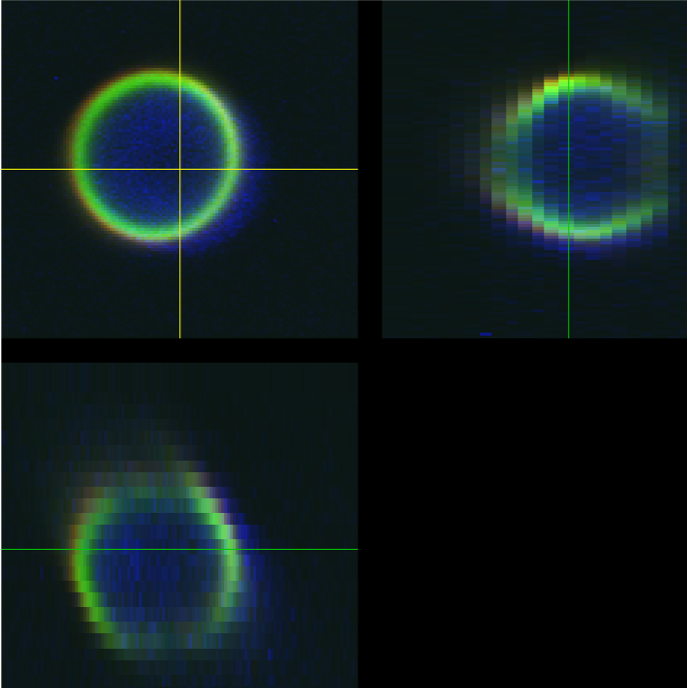
Before proceeding with the co-registration analysis, it is recommended to first check the XZ or YZ projection views of the datasets for any obvious signs of non-spherical or asymmetric aberration, which might indicate an issue with the system optics or alignment.
For microscopes used for colocalization experiments, it is recommended to run this protocol at least after installation and maintenance.
Expected result
Figure 2: Visual representation and quantification of different co-registration accuracy outcomes. Starting with a real dataset exhibiting an optimal level of co-registration (A), different levels of mis-registration in B and C were simulated by purposefully shifting one channel image of the bead relative to the other. Panel (A) shows an optimal co-registration of a single bead imaged in the middle of the FOV, characterized by precise alignment across all spatial axes (X, Y, Z). Panel (B) represents a minor co-registration shift along the X-axis (0.179 µm), characterized by a slight misalignment that may require minor adjustments or post-acquisition image processing to correct. Panel (C) illustrates a severe mis-registration shift along the Z-axis (0.599 µm), marked by a significant focal displacement between these channels. Under such conditions, steps must be taken to account for this mis-registration if conducting any co-localization or channel intensity ratiometric analyses either by system realignment, post-acquisition image registration correction, or simply excluding the region of the FOV where this bead resides for any of these types of analyses. The analysis of these real and simulated datasets was performed using MetroloJ_QC (version 1.3.1.1).
Here are the main steps to follow if you are using MetroloJ_QC plugin (version 1.3.1.2) on ImageJ :
Launch ImageJ (or Fiji) and open the MetroloJ_QC toolbar (Plugins > MetroloJ_QC)
Open your 3D multichannel stack (single 1 µm bead, 4 channels)
Click on the Co-registration Tool icon
Note
Before launching the MetroloJ_QC plugin, check the noise in the different channels. If needed, apply a median filter (radius 2-3) and a Substract background (radius 50). Noise is more prone to be seen in the blue channel.
In the Microscope Acquisition Parameters:
Choose the microscope type (CLSM), the objective specification, the pinhole size, and the excitation wavelengths.
In the Bead Detection Options:
Choose a thresholding method ("Minimum" is advised for noisy images);
Select “Centroid” as the center detection method;
Enable “Discard bead if more than one particle is thresholded". Set the background annulus size (for signal-to-background calculation);
Return to the main window, select "PDF report" and "Excel spreadsheet" in the "File Save Options", and run the analysis.
The tool will compute three useful metrics :
Shifts in X, Y, Z between all channel pairs: These represent the pixel distances between the bead centers in each channel pair along the X, Y, and Z axes. They quantify how misaligned the channels are in each spatial dimension.
Center-to-center distances: This refers to the 3D Euclidean distance between the centers of beads in two different channels. It combines the X, Y, and Z shifts into a single value and is calculated as:
Distance ratios relative to the reference resolution : This is the ratio of the measured center-to-center distance to the theoretical resolution of the microscope in the angle of the shift.
It helps assess how significant the shift is relative to the system’s resolution.
A ratio < 1 indicates acceptable co-registration; a ratio > 1 suggests potential misalignment beyond the system’s resolving capability
Citation
LINK
Profile view images (XY, XZ, YZ) and outlines of the thresholded bead will be shown for visual inspection.
If your images exhibit any misregistration, you can refer to the troubleshooting section for guidance.
Supplementary Information
Beads Selection
Different bead sizes can be used to assess co-registration accuracy in microscopy systems. Multi-color TetraSpeck beads of sizes 0.1, 0.2, 0.5, 1, and 4 µm are commercially available. We evaluated the performance of Tetraspeck 0.2, 1, and 4 µm beads side by side across 12 microscopes, with testing conducted by 11 members of the Quarep-LiMi WG4. Data analysis was performed using MetroloJ_QC (version 1.3.1.2), a plugin for Fiji/ImageJ software.
The green channel was used as the reference to determine the distance to the far-red (Ch0), red (Ch1), and blue (Ch3) channels. Our results indicate that 1 and 4 µm TetraSpeck beads have comparable performance, providing consistent measurements in the XY and Z-axis (Figures 3, 4, and 5). In contrast, Tetraspeck 0.200 µm beads exhibit higher variability and dispersion in measurements across all channels, particularly along the Z-axis (Figures 3B, 4B, and 5B), likely due to their lower achievable signal levels compared to the larger bead sizes. Additionally, 0.2 µm beads may be more prone to forming clumps that can be difficult to identify during image acquisition.
Figure 3: Lateral (XY) and axial (Z) distances were measured between far-red and green channels (Ch0) in µm on different bead sizes (4, 1, and 0.2 µm). Voxels are 0.070 x 0.070 x 0.200 µm. Measurements have been made by 11 WG04 Quarep members on more than 12 microscopes.
Figure 4: Lateral (XY) and axial (Z) distances were measured between red and green channels (Ch1) in µm on different bead sizes (4, 1, and 0.2 µm). Voxels are 0.070 x 0.070 x 0.200 µm. Measurements have been made by 11 WG04 Quarep members on more than 12 microscopes.
Figure 5: Lateral (XY) and axial (Z) distances were measured between blue and green channels (Ch3) in µm on different bead sizes (4, 1, and 0.2 µm). Voxels are 0.070 x 0.070 x 0.200 µm. Measurements have been made by 11 WG04 Quarep members on more than 12 microscopes.
For the 0.2 µm beads, two different sampling metrics were tested: 0.016 x 0.016 x 0.040 µm and 0.070 x 0.070 x 0.200 µm (Figures 6, 7, and 8). The results showed that smaller voxel sizes yield more precise and robust distance measurements to the reference channel. The SBR was comparable between the two voxel sizes, indicating that the primary difference was in the number of voxels and, consequently, the number of photons.
Figure 6: (A) Lateral (XY) and (B) axial (Z) distances were measured between far red and green channels (Ch0) in µm on 0.2 µm bead sizes. Voxels are 0.070 x 0.070 x 0.200 µm and 0.016 x 0.016 x 0.040 µm. Measurements have been made by 11 WG04 Quarep members on more than 12 microscopes.
Figure 7: (A) Lateral (XY) and (B) axial (Z) distances were measured between red and green channels (Ch1) in µm on 0.2 µm bead sizes. Voxels are 0.070 x 0.070 x 0.200 µm and 0.016 x 0.016 x 0.040 µm. Measurements have been made by 11 WG04 Quarep members on more than 12 microscopes.
Figure 8: (A) Lateral (xy) and (B) axial (z) distances were measured between blue and green channels (Ch3) in µm on 0.2 µm bead sizes. Voxels are 0.070 x 0.070 x 0.200 µm and 0.016 x 0.016 x 0.040 µm. Measurements have been made by 11 WG04 Quarep members on more than 12 microscopes.
The co-registration distance relative to the microscope’s theoretical resolution was calculated for all bead sizes. As shown in Figures 9A, 9B, and 9C, for the 4 µm and 1 µm beads, the ratios are below the system’s theoretical resolution, indicating that they are performing correctly with respect to co-registration. For the 0.2 µm beads, the data show greater dispersion; however, the majority of the analyzed beads fall within the reference ratio of 1. The same data are also represented in Figure 9D, where the distance ratio between the blue–green (B–G) channel and the red–green (G–R) channel is shown for all beads, and the Figure 9E, where the distance ratio between the Far red–green (G-FR) channel and the red–green (G–R) channel is shown for all beads. The green region indicates values with acceptable co-registration. In this representation, the beads with a ratio greater than 1 are easy to track, and it becomes clearer that the 0.2 µm beads are indeed problematic when analyzing the blue–green and the far red-green distances.
Figure 9: A, B, and C: Co-registration distance ratio between far-red and green (A), red and green (B), and blue and green (C), on different bead sizes (4, 1, and 0.2 µm). Voxels are 0.070 x 0.070 x 0.200 µm. D: Co-registration distance ratio between blue-green (B-G) channel compared to the red-green (G-R) channel of all the beads (4, 1, and 0.2 µm). The green area shows the accepted co-registration values. E: Co-registration distance ratio between the Far red–green (G-FR) channel compared to the red-green (G-R) channel of all the beads (4, 1, and 0.2 µm). The green area shows the accepted co-registration values. Measurements have been made by 11 WG04 Quarep members on more than 12 microscopes.
Despite the higher standard deviation observed with the Tetraspeck 0.2 µm beads, the average distances calculated to the reference channel were similar across all three bead sizes and the two voxel sizes.
Several parameters influence the ability to localize a bead, including its size, brightness, and the microscope's point spread function (PSF). The higher standard deviation observed with Tetraspeck 0.2 µm beads may result from their relatively weak fluorescence signal, as they contain fewer fluorescent molecules, which can lead to a low SBR and makes localization analysis more challenging. In contrast, due to their larger volume, 1 and 4 µm beads produce stronger fluorescence signals that improve the SBR, facilitating more precise localization analysis.
Although smaller beads, such as the Tetraspeck 0.2 µm, enable higher localization precision, we recommend using Tetraspeck 1 µm beads for routine co-registration analysis, as they yield higher SBR and provide more stable and reliable results, as our findings indicate. Therefore, 1 µm beads are better suited for routinely assessing the co-registration performance of microscopy systems, particularly in high-resolution systems where strong signal intensity is crucial, such as confocal laser scanning microscopes.
Of note, if localization precision is a key factor for a specific application, smaller diameter beads, such as the Tetraspeck 0.2 µm beads, should be used, guaranteeing that a sufficiently high SNR can be achieved. If a system is equipped only with low magnification objectives, the Tetraspeck 4 µm would be preferable.
Citation
LINK
Citation
LINK
Protocol references
Monitoring the point spread function for quality control of confocal microscopes V.1
Citations
Step 6.3
Amos, B, McConnell, G, Wilson, T. 2.2 Confocal Microscopy
https://doi.org/10.1016/B978-0-12-374920-8.00203-4Step 6.3
Wilhelm, S, Simbürger E, Bergter, A. Basics of Confocal Laser Scanning Microscopy ZEISS
https://www.zeiss.com/microscopy/en/c/lsc/24/confocal/basics-of-confocal-laser-scanning-microscopy-white-paper.htmlStep 9.3
Faklaris O, Bancel-Vallée L, Dauphin A, Monterroso B, Frère P, Geny D, Manoliu T, de Rossi S, Cordelières FP, Schapman D, Nitschke R, Cau J, Guilbert T. Quality assessment in light microscopy for routine use through simple tools and robust metrics.
https://doi.org/10.1083/jcb.202107093Acknowledgements
The authors thank Thya Delattre for highly valuable assistance in curating, processing, and analyzing the contributors' data. The authors thank Alexandra Palmer for contributing to this work with bead acquisition.