May 30, 2025
Development of a Machine Learning Model for Wellbore Stability Prediction Using Wire-Line Log Data and Drilling Parameters
- Mohatsim Mahetaji1
- 1Parul Institute of Technology, Parul University, Vadodara


External link: http://mohatsim786/wellbore-profile-prediction (github.com)
Protocol Citation: Mohatsim Mahetaji 2025. Development of a Machine Learning Model for Wellbore Stability Prediction Using Wire-Line Log Data and Drilling Parameters. protocols.io https://dx.doi.org/10.17504/protocols.io.81wgbkbd1gpk/v1
License: This is an open access protocol distributed under the terms of the Creative Commons Attribution License, which permits unrestricted use, distribution, and reproduction in any medium, provided the original author and source are credited
Protocol status: Working
We use this protocol and it's working
Created: May 24, 2025
Last Modified: May 30, 2025
Protocol Integer ID: 218881
Keywords: Wellbore Stability, Real-time monitoring, Reinforcement Learning, Machine Learning, Geomechanics , Petroleum Exploitation , predicting wellbore instability indicator, wellbore stability prediction, intelligent drilling operation, wellbore instability indicator, machine learning model, drilling parameter, drilling parameters this protocol, drilling engineer, supervised machine learning model, borehole breakout, such as borehole breakout, feature engineering, model training, line log data, multiple regression algorithm, line logging, using multiple regression algorithm, dataset
Disclaimer
This protocol is intended solely for academic and research purposes. The machine learning models and methods described herein are developed using publicly available datasets and are not designed or certified for direct application in live drilling operations without further validation. The author does not accept responsibility for any operational decisions made based on this protocol without proper engineering oversight, domain expertise, and site-specific analysis.
Users are advised to validate the model performance and predictions against actual field data and consult qualified drilling and geomechanics professionals before applying these techniques in real-world scenarios. The accuracy and reliability of the models may vary depending on geological complexity, data quality, and operational conditions.
Abstract
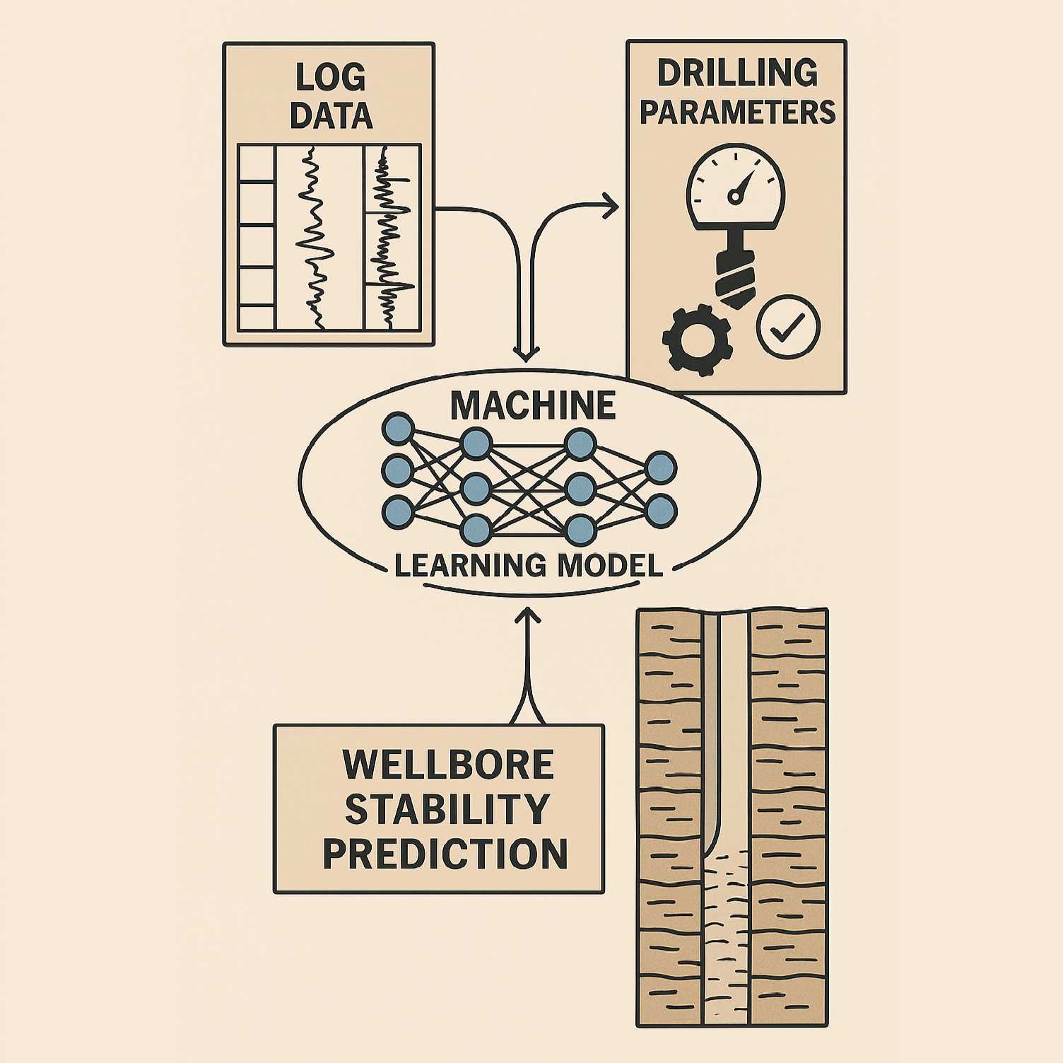
This protocol outlines the step-by-step methodology for building a supervised machine learning model aimed at predicting wellbore instability indicators—such as borehole breakout—based on wire-line logging and drilling parameters. The methodology integrates data acquisition from public datasets, preprocessing and feature engineering, model training using multiple regression algorithms, and interpretability using SHAP. The protocol is intended to serve geoscientists, drilling engineers, and data scientists interested in sustainable and intelligent drilling operations.
Attachments

Flow chart.png
1.6MB
Image Attribution
Source: OpenAI (ChatGPT / DALL·E image generation)
Guidelines
To ensure accurate and reproducible results when following this protocol, the following guidelines are recommended:
Data Integrity
- Use well-log and drilling datasets with consistent depth intervals and reliable measurement units.
- Validate and clean the data to remove null values, outliers, or inconsistencies before modeling.
Feature Selection
- Include input features that are physically relevant to wellbore stability, such as mechanical log parameters (e.g., GR, DTC, DTS, Density), directional data (e.g., Azimuth, Inclination), and drilling parameters (e.g., WOB, RPM, ROP).
- Avoid using highly collinear features together unless dimension reduction techniques are applied.
Model Training
- Ensure proper data scaling and normalization before feeding data into machine learning models.
- Use cross-validation to prevent overfitting and ensure robustness.
Ethical Use
- This protocol should not replace expert judgment or field engineering standards. It should serve as a supplementary analytical tool.
Materials
Programming Language: Python (v3.8+)
Software/Platforms: Jupyter Notebook, Google Colab or Anaconda
Hardware: A PC with a minimum of 8 logical processors (e.g., Intel i7/Ryzen 7) and at least 8 GB of RAM is recommended for developing and training machine learning models.
Libraries:
pandas, numpy, matplotlib, seaborn ,scikit-learn, XGBoost, SHAP (for model interpretation)
Data Source
Website: NLOGMapviewer - Q10-06 Well
Data Accessed: Wire-line logs, drilling parameters, and well trajectory information for Q10-06 well, Q10-A field, Netherlands.
Field Operator: Tulip Oil Netherlands Offshore B.V.
Drilling Dates: Start - 05 August 2015 | End - 21 September 2015
Well Type: Appraisal hydrocarbon
Well Status: Plugged back and sidetracked
Well Result: Gas with oil shows
Well Identification Details
Well Name: Q10-06
Location (WGS84): 52.4957164, 4.21468919
Delivered Location (ED50-GEOGR): 4.216013, 52.496498
End Depth: 2474 m (RT)
Vertical Depth: 2442.11 m (RT), 2402.01 m (MSL)
Rotary Table Elevation: 40.00 m (relative to MSL)
Trajectory: Deviated
Drilling Rig: Paragon C20052
Drilling Contractor: Paragon Offshore (North Sea) Ltd
Safety warnings
Before Applied to Real-Time: This protocol is designed for academic and research purposes only. Do not apply the model outputs directly in live drilling operations without field-specific validation and expert review.
Data Quality Sensitivity: The accuracy of predictions is highly dependent on the quality, consistency, and completeness of the input data. Incomplete or poorly processed data can lead to misleading results.
Overfitting Risk: Improper model tuning or training on unbalanced data may result in overfitting, leading to poor generalization on unseen data.
Misinterpretation of SHAP Values: SHAP outputs show statistical feature influence, not causality. Misinterpretation may lead to incorrect engineering conclusions.
Empirical Assumptions Avoided: While this protocol avoids empirical correlations, the models still rely on assumptions within machine learning algorithms. Interpret results with caution.
Ethics statement
This research does not involve experiments on animals or human subjects. Therefore, prior approval from an Institutional Animal Care and Use Committee (IACUC) or equivalent ethics committee was not required. However, all data used in this study were obtained from publicly accessible sources with proper authorization, ensuring compliance with applicable data use policies and ethical guidelines.
Before start
- Ensure Python 3.8+ is installed along with required libraries: pandas, numpy, scikit-learn, xgboost, shap, etc.
- Download well data.
- Use a system with at least 8 logical processors and 8 GB RAM for model training.
- Familiarity with machine learning regression and Python (e.g., Jupyter Notebook) is recommended.
- Prepare data in structured CSV/Excel format with consistent depth intervals.
Procedure: 1.0 Data Collection and Preprocessing
Data Source:
- Wire-line log and drilling data were collected for the well from the publicly accessible NLOG database (https://www.nlog.nl).
- The well spans from 2177.80 m to 2350.92 m depth with a total of 1137 data points at 0.15 m intervals.
input Features:
The selected 17 input features include:
MD, TVD, Inclination, Azimuth, X-offset, Y-offset, Bit Size, GR, NPHI, DTC, DTS, Density, Deep/ Shallow Resistivity, ROP, WOB, RPM.
Output Label:
The Caliper log was used as the target variable representing borehole diameter to detect breakouts.
Preprocessing Steps:
- Null values were handled using linear interpolation or filled with the median.
- Numerical features were standardized using StandardScaler.
- Data was split into training and testing sets in an 80:20 ratio.
Procedure: 2.0 Feature Engineering
Transformation:
- Polynomial features (second-order) were generated for models like Polynomial Regression.
- Directional features such as (X-offset – Y-offset) were considered to represent trajectory-driven stress shifts.
- Statistical checks for multicollinearity were applied using VIF analysis.
Procedure: 3.0 Model Selection and Training
Model List:
Twelve supervised regression models were developed and evaluated:
- Linear Regression
- Polynomial Regression (Degree 2)
- Gradient Boosting Regressor (GBR)
- Histogram Gradient Boosting (HGB)
- Random Forest Regressor (RFR)
- Decision Tree Regressor (DTR)
- Support Vector Regression (SVR)
- Gaussian Process Regressor (GPR)
- Bernoulli Naive Bayes (BNB)
- Gaussian Naive Bayes (GNB)
- K-Nearest Neighbors (k-NN)
- Multi-Layer Perceptron (MLP)
Training & Optimization:
- Scikit-learn’s train_test_split function was used.
- Models were tuned using GridSearchCV where applicable.
- Feature scaling and normalization were ensured before model feeding.
Procedure: 4.0 Cross-Validation and Evaluation
Validation Method:
For each model, performance was recorded using:
- Root Mean Squared Error (RMSE)
- Determination Coefficient (DC / R²)
- Error Distribution Metrics: Mean error %, Standard Deviation (σ), Kurtosis, Skewness.
Procedure: 5.0 SHAP (SHapley Additive Explanations)
Model Interpretability:
shap.explainer() from the SHAP library was used for model interpretation.
SHAP Summary and Force plots were generated for each model to evaluate the relative contribution of input features.
For example, Gradient Boosting showed that azimuth, inclination, and GR were strong predictors of breakout.
Procedure: 6.0 Result Recording and Visualization
Histogram Analysis:
- Histograms of the percentage error distribution were plotted to identify model biases.
- Kurtosis and Skewness were used to assess distribution behavior.
Model Comparison:
After training all selected machine learning models, a systematic comparison process was carried out. Each model’s predictions were evaluated using consistent metrics, including Root Mean Square Error (RMSE), determination coefficient (R²), and statistical error analysis parameters such as mean error percentage, standard deviation, kurtosis, and skewness.
Visual tools such as error histograms were used to analyze prediction distribution patterns and detect tendencies toward overfitting or underfitting. Models were assessed not only for predictive accuracy but also for consistency and robustness across the full depth range.
The comparison process involved examining the shape of the prediction error distribution, identifying symmetric or skewed behavior, and evaluating whether the distribution matched expected physical patterns in the data. Feature importance was also evaluated using SHAP plots to understand which input parameters had the most influence on each model’s predictions.
This structured comparison framework ensured an objective and reproducible approach for selecting the most appropriate models for the given geomechanical prediction task.
Protocol references
Mahetaji, M. and Brahma, J., 2024. A critical review of rock failure Criteria: A scope of Machine learning approach. Engineering Failure Analysis, 159, p.107998.https://doi.org/10.1016/j.engfailanal.2024.107998
Su, X., Yan, X., & Tsai, C. L. (2012). Linear regression. Wiley Interdisciplinary Reviews: Computational Statistics, 4(3), 275–294. https://doi.org/10.1002/WICS.1198
Suykens, J. A. K., & Vandewalle, J. (1999). Least squares support vector machine classifiers. Neural Processing Letters, 9(3), 293–300. https://doi.org/10.1023/A:1018628609742/METRICS
Kor, K., Ertekin, S., Yamanlar, S., & Altun, G. (2021). Penetration rate prediction in heterogeneous formations: A geomechanical approach through machine learning. Journal of Petroleum Science and Engineering, 207, 109138. https://doi.org/10.1016/J.PETROL.2021.109138
Mohamadian, N., Ghorbani, H., Wood, D. A., Mehrad, M., Davoodi, S., Rashidi, S., Soleimanian, A., & Shahvand, A. K. (2021). A geomechanical approach to casing collapse prediction in oil and gas wells aided by machine learning. Journal of Petroleum Science and Engineering, 196, 107811. https://doi.org/10.1016/J.PETROL.2020.107811
Radwan, A. E. (2022). Drilling in Complex Pore Pressure Regimes: Analysis of Wellbore Stability Applying the Depth of Failure Approach. Energies 2022, Vol. 15, Page 7872, 15(21), 7872. https://doi.org/10.3390/EN15217872
Hao, J. and Ho, T.K., 2019. Machine learning made easy: a review of scikit-learn package in python programming language. Journal of Educational and Behavioral Statistics, 44(3), pp.348-361. https://doi.org/10.3102/1076998619832248
Marcílio, W.E. and Eler, D.M., 2020, November. From explanations to feature selection: assessing SHAP values as feature selection mechanism. In 2020 33rd SIBGRAPI conference on Graphics, Patterns and Images (SIBGRAPI) (pp. 340-347). Ieee. DOI: 10.1109/SIBGRAPI51738.2020.00053
Mahetaji, M. and Brahma, J., 2024. Prediction of minimum mud weight for prevention of breakout using new 3D failure criterion to maintain wellbore stability. Rock Mechanics and Rock Engineering, 57(3), pp.2231-2252. https://doi.org/10.1007/s00603-023-03679-4
Acknowledgements
I gratefully acknowledge the Netherlands Oil and Gas Portal (NLOG), operated by TNO Geological Survey of the Netherlands, for providing open access to well data and supporting resources. The wire-line log data and drilling parameters for the Q10-06 well used in this study were retrieved from the NLOG Mapviewer. I commend NLOG's commitment to transparency and data sharing, which significantly contributes to academic and industrial research in subsurface exploration and development.