Oct 23, 2020
Detection and Sorting of Extracellular Vesicles and Viruses using nanoFACS
- Aizea Morales-Kastresana1,
- Joshua Welsh1,
- Jennifer Jones1
- 1Translational Nanobiology Section, Laboratory of Pathology, Center for Cancer Research, National Cancer Institute, National Institutes of Health
- Translational Nanobiology Section


Protocol Citation: Aizea Morales-Kastresana, Joshua Welsh, Jennifer Jones 2020. Detection and Sorting of Extracellular Vesicles and Viruses using nanoFACS. protocols.io https://dx.doi.org/10.17504/protocols.io.bj6xkrfn
License: This is an open access protocol distributed under the terms of the Creative Commons Attribution License, which permits unrestricted use, distribution, and reproduction in any medium, provided the original author and source are credited
Protocol status: Working
We use this protocol and it's working
Created: August 22, 2020
Last Modified: October 23, 2020
Protocol Integer ID: 40887
Keywords: Astrios EQ, jet-in-air, small particle, flow cytometry, extracellular vesicles, flow virometry, nanoFACS, nanofacs recent advances in high resolution flow cytometry, specific ev surface protein, sorting of extracellular vesicle, high resolution flow cytometry, extracellular vesicle, fluorescence sensitivity, antibody, antibodies in basic protocol, antibody removal, using nanofac, specific staining with fluorochrome, dc markers such as mhc, low expression of typical dc marker, label ev, conjugated antibody, negative control for antibody, dc marker, typical dc marker, antigen,
Disclaimer
This protocol summarizes key steps for a specific type of assay, which is one of a collection of assays used for EV analysis in the NCI Translational Nanobiology Section at the time of submission of this protocol. Appropriate use of this protocol requires careful, cohesive integration with other methods for EV production, isolation, and characterization.
Abstract
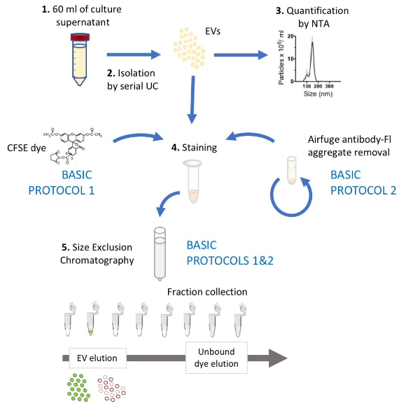
Recent advances in high resolution flow cytometry (HRFC), which show improvements in both light scatter and fluorescence sensitivity have resulted in the development of techniques that better isolate, stain and analyze single EVs(Boing et al., 2014; Groot Kormelink et al., 2016; Morales-Kastresana, Musich, Welsh, Telford, Demberg, Wood, Bigos, Ross, Kachynski, Dean, Feton, et al., 2019; Morales-Kastresana et al., 2017; Stoner et al., 2016; van der Vlist, Nolte-'t Hoen, Stoorvogel, Arkesteijn, & Wauben, 2012). Below, we describe protocols to fluorescently label EVs using CFDA-SE (hereinafter called CFSE), as well as antibodies targeted at specific EV surface proteins. We also provide guidelines for residual dye and antibody removal, appropriate data acquisition by HRFC and EV counting by HRFC. Figure 1summarizes these protocols.
The EVs used in this protocol are derived from the DC2.4 cell line, and bone marrow derived dendritic cells (BMDCs). The DC2.4 cell line are immature dendritic cells (DCs) with very low expression of typical DC markers on their surface (unpublished observation and(Hargadon, Forrest, & Reddy, 2012)) and that release a morphologically homogeneous population of EVs (~130 nm in diameter). DC2.4 EVs will be used to demonstrate a CFSE staining in Basic Protocol 1, as well as being used as a negative control for antibody-based staining methods (Basic Protocol 2). Bone marrow dendritic cell (BMDC)-derived EVs are more heterogeneous in diameter (100-200 nm) and composition(Morales-Kastresana, Musich, Welsh, Telford, Demberg, Wood, Bigos, Ross, Kachynski, Dean, Felton, et al., 2019), and express DC markers such as MHC-II. BMDC EVs will be used to demonstrate antigen-specific staining with fluorochrome-conjugated antibodies in Basic Protocol 2. DC2.4 and BMDC-derived EVs were isolated by serial ultracentrifugation, with concentration and diameter distribution characterized by NTA, as described before(Morales-Kastresana, Musich, Welsh, Telford, Demberg, Wood, Bigos, Ross, Kachynski, Dean, Feton, et al., 2019; Morales-Kastresana et al., 2017).
Basic Protocol 1
Prepare 15 µL of DPBS containing between ~1x10⁸ to ~2.5 x 10⁹ DC2.4-derived EVs in a 1.7 ml microfuge tube.
Note
Note: This number of EVs correspond to ~ 0.1-2.5 µL of EV stock, if prepared as described previously(Morales-Kastresana et al., 2017), starting with 60 ml of supernatant from cells cultured for 48h in EV depleted medium. The reaction volume and CFSE concentrations are optimized for staining approximately 1x10⁹EVs. The use of different EV numbers may therefore result in suboptimal staining. When larger amounts of labeled EVs are required, this protocol can be scaled up with similar results.
In a separate 1.7 ml microfuge tube, prepare 15 µL of DPBS containing 80 µM of CFDA-SE, from a 10 mM stock solution of CFDA-SE in DMSO. For this, add 0.12 µL of 10 mM CFDA-SE in 15 µL of DPBS. Intermediate dilutions in DPBS may be prepared to facilitate the dilution process.
Note
Note: It is recommended to store the CFDA-SE stock reconstituted in DMSO in small aliquots at -80ºC. Avoid using DPBS or other aqueous solutions for storing purposes, since aqueous solutions favor the hydrolysis of diacetic groups in CFDA-SE and therefore decrease the permeability of the dye and incorporation into EVs(Banks et al., 2013; Bergsdorf et al., 2003; Hoefel et al., 2003). Also due to this risk of hydrolysis, it is critical for the aliquots to be stored in an anhydrous manner. If the EV number and reaction volume are scaled up in step 1, scale up the CFDA-SE quantity, so as to achieve an 80 µM CFDA-SE solution.
Pipette the CFDA-SE solution on top of the EV solution. Mix the solution by pipetting and incubate for two hours at 37ºC in the dark. The incubated CFSE concentration is now 40 µM.
Note
Note: The incubation time may be extended to increase CFDA-SE’s incorporation into EVs. However, the authors have observed a decrease in the EV number after long incubation periods(Morales-Kastresana et al., 2017).
15 minutes before the incubation completion time, wash a NAP-5 size exclusion chromatography (SEC) column with 10 ml of DPBS. Never allow the column to dry.
Note
Note: To automate the washing process, a pump can be setup to help add DPBS onto the column.
Prepare collection tubes for the collection of two fractions. To facilitate the visualization of eluted sample, use a marker pen to draw a line indicating the 500 µL mark on each collection tube.
Note
Note: The first fraction is the “dead volume,” of buffer alone, that elutes before fractions containing material from the loaded sample. The majority of DC2.4 EVs appear in fraction 2. Some EVs may however elute in fraction 3. Free dye elutes in fractions ~7-8.
When the two-hour incubation period is complete, increase the CFSE-stained EV preparation volume to 100 µL by adding 70 µL of DPBS and mix by pipetting.
Note
Note: If the staining is scaled up in step 1 to increase the number of EVs, then add DPBS to a final volume of 100 µL. If the total volume is higher that 100 µL, use multiple columns to wash the sample.
Pipette the 100 µL of CFSE-stained EVs on to the SEC column and immediately start collecting 500 µL fractions.
When the 100 µL of sample has completely entered the column bed, add 500 µL of DPBS and continue collecting fractions. ~80% of the eluted EVs will be collected in fraction 2.
Representative contour plots of unstained and CFSE-stained DC2.4 EV (before and after SEC). The number of fluorescein molecules incorporated in the EVs is shown in the plot (protocol for calculating the MESF is described in Basic Protocol 6). Red box indicates system reference noise.
Basic Protocol 2
Protocol
CREATED BY
Jennifer Jones
Wash one qEV column per EV preparation with 20 mL of DPBS. Never allow the columns to become dry.
Pipette 1x10⁹EVs in a 10 µL volume of DPBS and add 2 µg of Fc Block reagent to block Fc receptors. Incubate with no agitation for 10 minutes at room temperature.
Note
Note: The presence of Fc receptors on EVs is not well documented. However, adding Fc Block will not only block putative Fc receptors, but also serves as a source of protein to block other non-specific binding sites of fluorescent antibodies.
In a 1.7 mL microfuge tube, pipet 1.5 µg of fluorochrome-conjugated antibody and add DPBS to a finale volume of 120 µL per sample. Mix by pipetting up and down. Prepare a master mix if multiple samples are to be stained with the same antibody.
Note
Note: This antibody quantity is a reference starting point when testing a new antibody. Antibody titration is recommended to achieve optimal staining and avoid the use of unnecessary material. Many anti-human antibodies are provided in a test volume format (µL per test) rather than in concentration (µg mL-1).
Transfer the 120 µL of the antibody solution to an airfuge tube and mark one side of the tube with a waterproof marker. Place the tube with a corresponding balance into an A100/18 rotor, with the mark facing up. Place a lid on the rotor.
Note
Note: The mark is a reference for the location of the antibody aggregates after airfuging. Using the rotor cover can reduce sample evaporation during centrifugation.
Place the rotor into the airfuge and close the airfuge lid tightly. Open the air source to centrifuge until the gauge reads 22 psi (~130,000 RCF) and leave for 5 minutes.
Note
Note: In order to avoid extreme heat during centrifugation, airfuge step can be performed in a cold room. Alternatively, the authors cool down the rotor before using it.
When the airfuge step is complete, use sharp tweezers to remove the tubes from the rotor and place them on the corresponding rack.
Gently pipet off the top 70 µL of solution and add it on top of the EV solution.
Note
Note: Antibody aggregate pellets cannot always be observed. For that reason, leaving a reasonable volume in the bottom of the tube and using the top part of the solution is recommended.
Incubate the EVs with antibody 15-30 minutes in the dark at room temperature whilst being gently agitated.
Note
Note: As with CFSE, time is a parameter that can be modulated to increase the labeling with antibodies. The authors have observed slight improvements of staining with certain epitopes when increasing the staining period up to 1 hour.
Prepare collection tubes for 12 fractions. To facilitate the visualization of eluted sample, use a marker to draw a line indicating the volume of each fraction (500 µL) on the side of the collection tubes.
Add DPBS to the EV prep to a final volume of 500 µL and proceed to remove unbound antibody using SEC with qEV columns. Samples that are not going to be immediately loaded on the columns can be stored at in the dark at 4ºC.
Wait until all of the DPBS used for pre-washing the column has entered the column bed. Immediately load 500 µL of the sample and simultaneously start collecting 500 µL fractions.
Keep adding DPBS (500 µL each time) and whilst collecting fractions. Stained EVs will start eluting in fraction 7, with the majority in fractions 8-9. For maximum recovery, harvest fraction 10 too.
Store EVs at 4ºC and in the dark until performing flow cytometric analysis. Alternatively, some antibody-fluorochrome conjugates can resist one freeze/thaw cycle and therefore, labeled EVs can be stored at -80ºC if being analyzed at a later date.
qEV columns can be stored at 4ºC and reused with extensive washing. Authors recommend washing them with a minimum 50 ml of DPBS, to elute as much remaining antibody as possible, followed by 10 ml of 20% ethanol diluted in DPBS to keep the columns aseptic during storage. When reusing a column, wash 40 ml of DPBS to make sure that any traces of ethanol are removed.
Proceed to analysis.
Representative contour plots show PBS, unstained, and MHCII-stained BMDC EV (before and after SEC) and control DC2.4 EVs that lack of MHCII on their surface. Red box indicates system reference noise.
Basic Protocol 3
Turn on the instrument at least an hour before running the samples. Let the pressure and stream to stabilize and prime the fluidics system to remove bubbles in the circuit. Turn lasers on and allow them to warm up whilst shuttered.
Wash the sample line with FACS Rinse solution for about 20 minutes at a high differential pressure (1 psi over the sheath pressure). Repeat same procedure with clean DPBS for 20 more minutes.
Adjust the vertical alignment.
Note
Note: To test whether the stream is vertical or not, raise the nozzle while looking at the relative position of the stream to the pinholes. If the position doesn’t change, the stream is vertically well aligned; if it does change, then the verticality must be tweaked. A good vertical alignment maximizes the detection of parameters in all laser paths.
Set the triggering threshold to the 561-SSC channel. Adjust the triggering threshold channel and voltage to allow the visualization of the noise population, to approximately 10,000 events per second.
Note
Note: The noise is a random representation of the diffusely scattered photons from the laser beam and stream intercept.Because of the high event rate of these low-level signals, inclusion of these events on some instruments is only feasible in a very limited way due to limitations in their baseline restoration algorithms and other signal processing attributes.Background noise is informative because: i) it serves as a window into the population of EVs that fall under the triggering-threshold; ii) it allows the determination of too much free dye in the interrogation point; and iii) it helps to identify when EV samples are being analyzed at a concentration that is too high and is therefore at risk of coincident detection(Morales-Kastresana et al., 2017; van der Pol, van Gemert, Sturk, Nieuwland, & van Leeuwen, 2012). For these reasons, the authors refer to the noise as “background reference noise”.
Load a sample containing a mix of 200 nm yellow and red beads at 1x10⁷beads ml-1(about a 1x10⁶-fold dilution of original stock) to fine-tune the stream:laser alignment.
Note
Note: Any combination of beads that are excited by different lasers can be used. The goal is to have two populations, whose fluorescence will be collected in different pinholes, in a way that the stream is aligned according to two pinholes. This ensures the correct vertical alignment.
Note
Note: The dimmer the fluorescent beads used, the better the alignment will be for EVs.
Open a dot plot depicting yellow (~515 nm) and red (~605 nm) fluorescent channels in each axis (or correspondent fluorescent axis for the chosen beads). Tweak the alignment until the fluorescence signal is optimized for both bead sets. While doing this, try to keep the total event rate, including the noise, around 10,000-20,000.
Note
Note: Alignment will be optimal when the distance between the noise and bead populations is the biggest in terms of fluorescence, while the bead population remains as tight as possible. Also, the event rate should not increase significantly with respect to DPBS alone, since the contribution of the beads to the overall rate is insignificant.
Note
Note: It is very useful to monitor Time versus any parameter (fluorescence and scatter) to determine how the distance between noise and beads varies with alignment adjustments.
Plots with the time parameter on the X-axis and scatter or fluorescent on the Y-axis during the alignment process to monitor the relative separation between the beads and noise (a). b and c show scatter and fluorescent parameters before (b) and after (c) optimizing the alignment. YB indicates 200 nm yellow fluorescent beads, RB indicates 200 nm red fluorescent beads.
Note
Note: If the bead populations and the reference noise population appear as “split” populations, there is probably drop-drive noise (especially with the 70 µm nozzle), which can be eliminated by dropping the break off point by lowering the amplitude or frequency, to the extent possible while maintaining stable Intelli-Sort settings and a stable breakoff point.
Once aligned, acquire and save a representative sample of the beads used for the alignment.
Note
This file will serve as a reference for future alignment, allowing comparisons between the alignment between experiments.
Wash the sample line with DPBS for 5 minutes at 1 psi.
Note
Note: As the sample lines clear, monitor the disappearance of the 200 nm beads from the alignment steps over time by referring to the time versus scatter or fluorescence plots. If alignment beads do not disappear completely, increase the pressure up to a differential pressure of 1.4. If beads are still observed, there may be contaminating beads in the sample path (either in the lines, junction points between fittings, or in the nozzle reservoir), and you will need to clear these residual beads before continuing. It can be useful to wash the line with rinse solution and followed by DPBS for 5 minutes each. Once washing is done, change rinse and DPBS tubes for future uses, as these solutions may contain contaminating beads from the sample injection tube.
Save an acquisition of 30 seconds of clean DPBS.
Load the EV sample, increase pressure up to 1 psi to accelerate the sample loading and then decrease the differential pressure to 0.3 psi.
Note
Note: A 0.3 psi differential pressure is offered here as a reference for what commonly works on AstriosEQ sorters that we have worked with. A differential pressure that permits stable detection of single EVs, avoiding coincidence, should be selected. Authors recommend keeping the differential pressure the same for all samples to be analyzed during an experiment, since event rate can be a valuable source of information.
Wait until the event rate is stable (use the time versus scatter plot). Then stop the acquisition in the software (not the machine) and start acquiring again for 30 seconds. Save the acquisition.
Note
Note: Authors recommend saving acquisitions of the same duration, in order to compare event numbers among samples.
Wash the sample line with DPBS for 5 minutes at 1 psi.
Run samples, save acquisitions and wash with DPBS, as described above.Keep samples at 4°C and in the dark.
Wash the sample line with FACSClean, FACSRinse and DPBS consecutively, for 10 minutes each at 2 psi. Turn off the lasers and fluidics. Rinse the nozzle and place a FACS tube cap with some clean water under the nozzle tip.
| ARTIFACT | SOURCE | WHAT TO DO | |
| False positive signal | Drop drive noise | Reduce amplitude and/or frequency | |
| Nonspecific binding of antibodies | Add control EVs that do NOT express the target antigen | ||
| Antibody/dye aggregates | Add control EVs that do NOT express the target antigen | ||
| Add control antibody/dye alone | |||
| Background antibody/dye fluorescence | Add control antibody/dye alone | ||
| Noise fluorescence shifting | |||
| Low resolution of positive signal over the noise/negative population | Background antibody/dye fluorescence | Wash the excess antibody/dye | |
| No positive signal detection | Low antigen density | Use a more sensitive instrument, brighter fluorochrome and/or brighter staining method | |
| Low antibody affinity | Increase concentration and/or incubation time | ||
| Antibody/fluorochrome conjugate not working properly | Change antibody/clone/fluorochrome/lot | ||
| Unexpected increase in event rate | Change in differential pressure of sheath tank and sample line | Time vs scatter parameter to identify these peak | |
| Stuck material in sample line/nozzle | Flush sample line with detergent and PBS with increased sample pressure differential (boost). | ||
| Contaminating material from previous sample | Run filtered PBS before and after samples, to minimize the presence of contaminating particles. | ||
| Coincident detection of particles | Sample is too concentrated | Dilute the sample | |
| Use spike in beads to ensure an operational concentration range | |||
| Nanobubbles at the interrogation point | Are created due to the high pressure in the nozzle | Run PBS control between samples to have that source of noise identified and controlled |
A list of the most frequent artifacts observed by the authors is listed, along with a brief explanation and the suggested controls to consider, either to identify or to avoid such artifacts.
Basic Protocol 4
Protocol
CREATED BY
Jennifer Jones
Prepare a stock of 200 nm polystyrene reference beads by diluting 50 µL of Fluosphere beads in 50 ml of DPBS (1000-fold dilution) and keep this solution as a ‘Big Stock’. Determine the particle concentration of the beads in the ‘Big Stock’using NTA or any other method.
Note
Companies provide an estimated concentration of beads in solution, based on the size and weight. This tends to be a rough estimation, we therefore recommend preparing a 10,000x dilution of ‘Big Stock’ beads in DPBS to perform quantification of particles per ml. Polystyrene beads are stable in DPBS, with no significant loss of particles and fluorescence over time. Polystyrene particles can therefore be quantified once and used in the next couple of years. As a reference, the authors’ ‘Big Stock’ of 200 nm yellow-green beads listed in the Material section is at ~1.8 x 10¹⁰particles/ml, measured by NTA. It is worth noting that every time an aliquot is taken from the ‘Big Stock’ its concentration will likely decrease. It is therefore recommended that several smaller ‘Big Stock’ aliquots to ensure better consistency over long periods of time.
Vortex the bead stock solution for 5 seconds.
Prepare a working stock of beads by diluting them 100-fold in DPBS (~1.8 x 10⁸ particles/ml). Keep this working stock for the whole experiment.
Prepare EVs in a known volume of DPBS and annotate the dilution, if any. Note that if coming from Basic Protocols 1 and 2, expect some EV loss during the protocol and dilute accordingly.
Vortex the working stock of beads for 5 seconds.
Spike the beads by diluting them 100-fold in the EV prep. The final concentration of reference beads, if following previous example, will be 1.8 x 10⁶ particles/ml. Mix the sample.
Run the EV sample containing the spiked reference beads as described in Basic Protocol 4.
Note
200 nm polystyrene beads may overlap in scatter with some EVs. The authors therefore use 200 nm yellow-green beads if EVs are stained PE or APC, or 200 nm red beads if EVs are stained with CFSE or FITC. This allows differentiation of the EV and bead populations more easily and will provide a more reliable count.
Record the EV and bead event count as shown.
Note
The detectable concentration is dependent upon the limit of detection of the instrument and how the gating strategy was defined. In accordance with the MIFlowCyt-EV framework, parameters being used to gate EVs and the threshold of the instrument should be calibrated into standard units to allow the detectable concentration to be defined in standard units that can be validated(Welsh et al., 2020). See dx.doi.org/10.17504/protocols.io.bjcqkivw for information on how to calibrate fluorescence and light scatter parameters into standard units.
EV concentration of a solution can be calculated using beads as spike in references.a) nanoFACS plots depicting FSC and SSC signals in the 488 nm laser channel for control PBS, 200 nm polystyrene spike in beads and DC2.4 EVs + spike in beads. b) Determined concentration of DC2.4 EVs from nanoparticle tracking analysis and Astrios EV using calculated based on reference bead counts. Experiments were performed in triplicate (median ± 25th, 75thpercentile plotted for NTA and Astrios EQ data).
Multiply the EV count by the bead concentration before dividing by the bead count, as shown in the following equation:
Note
Note: If there is any noise or background source in the EV gate, these background counts must the subtracted to approximate EV counts. A clear example of this background would be any events that we get when running clean PBS. In that case use equation:
Further information
Background information, critical parameters, and troubleshooting steps can be found within the manuscript.