DeepClone, an end-to-end protocol to study somatic mutagenesis and selection at high resolution

Ferriol Calvet; Morena Pinheiro-Santin; Erika Lopez; Raquel Blanco Martinez-Illescas; Núria amper; Miguel L. Grau; Ferran Muiños; Rocío hamorro González; Maria Andrianova; Federica Brando; Stefano Pellegrini; Axel Rosendahl Huber; Marta Huertas; Elisabet Figuerola-Bou; Coohleen Coombes; Brendan F. Kohrn; Jeanne Fredrickson; Rosa Ana Risques; Nuria Lopez-Bigas; Abel Gonzalez-Perez

Jan 13, 2026

Version 1

DeepClone, an end-to-end protocol to study somatic mutagenesis and selection at high resolution V.1

DOI

https://dx.doi.org/10.17504/protocols.io.dm6gp1jodgzp/v1

DeepClone, an end-to-end protocol to study somatic mutagenesis and selection at high resolution

Ferriol Calvet^1,2,3,
Morena Pinheiro-Santin¹,
Erika Lopez^1,3,
Raquel Blanco Martinez-Illescas^1,2,3,
Núria amper¹,
Miguel L. Grau¹,
Ferran Muiños^1,3,
Rocío hamorro González¹,
Maria Andrianova¹,
Federica Brando¹,
Stefano Pellegrini^1,2,3,
Axel Rosendahl Huber^1,3,
Marta Huertas¹,
Elisabet Figuerola-Bou¹,
Coohleen Coombes⁴,
Brendan F. Kohrn⁴,
Jeanne Fredrickson⁴,
Rosa Ana Risques⁴,
Nuria Lopez-Bigas^1,2,3,5,6,
Abel Gonzalez-Perez^1,2,3,6

¹Institute for Research in Biomedicine (IRB Barcelona), The Barcelona Institute of Science and Technology, Baldiri Reixac, 10, 08028 Barcelona, Spain;
²Department of Medicine and Life Sciences, Universitat Pompeu Fabra, Barcelona, Spain;
³Centro de Investigación Biomédica en Red en Cáncer (CIBERONC), Instituto de Salud Carlos III, Madrid, Spain;
⁴Department of Laboratory Medicine and Pathology, University of Washington, Seattle, WA;
⁵Institució Catalana de Recerca i Estudis Avançats (ICREA), Barcelona, Spain;
⁶These authors jointly supervised this work: A. Gonzalez-Perez, N. Lopez-Bigas

Morena Pinheiro-Santin

IRB Barcelona

DOI: https://dx.doi.org/10.17504/protocols.io.dm6gp1jodgzp/v1

Protocol Citation: Ferriol Calvet, Morena Pinheiro-Santin, Erika Lopez, Raquel Blanco Martinez-Illescas, Núria amper, Miguel L. Grau, Ferran Muiños, Rocío hamorro González, Maria Andrianova, Federica Brando, Stefano Pellegrini, Axel Rosendahl Huber, Marta Huertas, Elisabet Figuerola-Bou, Coohleen Coombes, Brendan F. Kohrn, Jeanne Fredrickson, Rosa Ana Risques, Nuria Lopez-Bigas, Abel Gonzalez-Perez 2026. DeepClone, an end-to-end protocol to study somatic mutagenesis and selection at high resolution. protocols.io https://dx.doi.org/10.17504/protocols.io.dm6gp1jodgzp/v1

Manuscript citation:

Ferriol Calvet, Morena Pinheiro-Santin, Erika López-Arribillaga, Raquel Blanco Martinez-Illescas, Núria Samper, Miguel L. Grau, Ferran Muiños, Rocío Chamorro González, Maria Andrianova, Federica Brando, Stefano Pellegrini, Axel Rosendahl Huber, Marta Huertas, Elisabet Figuerola-Bou, Coohleen Coombes, Brendan F. Kohrn, Jeanne Fredrickson, Rosa Ana Risques, Nuria Lopez-Bigas@, Abel Gonzalez-Perez@. DeepClone, an end-to-end protocol to study somatic mutagenesis and selection at high resolution. Under review in Nature Protocols

License: This is an open access protocol distributed under the terms of the Creative Commons Attribution License, which permits unrestricted use, distribution, and reproduction in any medium, provided the original author and source are credited

Protocol status: Working

We use this protocol and it's working, but we are still developing and optimizing it

Created: January 07, 2026

Last Modified: January 13, 2026

Protocol Integer ID: 238161

Keywords: duplex sequencing, computational pipeline, DNA sequencing, normal tissue sequencing, deep sequencing, nextflow, cancer, molecular biology, library preparation, genomics, somatic mutation, mutation, DeepClone, molecule resolution, error rate, detection of somatic mutation, advent of next generation sequencing, somatic mutagenesi, multiple aspects of mutagenesi, interplay between mutagenesi, next generation sequencing, mutagenesi, somatic mutation, calculations of mutagenesi, sequencing technology, mutation calling, sequencing library preparation solution, mutational process, adoption of dna duplex, thousands of clone, sequencing, study of mutational process, dna, introduction of dna duplex, sequencing raw data, experimental dna duplex, dna duplex, somatic evolution in scenario, clone, understanding somatic evolution, salient clone, deepclone, cancer, generation, computational tool

Funders Acknowledgements:

Cancer Research UK

Grant ID: CGCATF-2021/100008

NCI

Grant ID: OT2CA278668

Disclaimer

We strongly encourage users to follow the steps from the attached PDF files. The steps provided here are the same ones as those in the PDF, but they may be missing some clarifications due to format restrictions.

Abstract

The advent of Next Generation Sequencing (NGS) technologies opened up the door to the study of somatic mutagenesis and selection through the analysis of a salient clone in a sample, as in the case of cancer. This was made possible by the development of an ecosystem of computational methods that enabled mutation calling, the study of mutational processes, and the quantification of positive selection, among other research avenues. Recently, the introduction of DNA duplex sequencing technologies has allowed the detection of somatic mutations that occur in one or few cells in a sample. This has unlocked the possibility to study the interplay between mutagenesis and selection on hundreds or thousands of clones per sample, providing access to understanding somatic evolution in scenarios that were not previously easy to access, such as normal tissues. The adoption of DNA duplex sequencing technologies has been hindered, among other reasons, by the lack of a complete ecosystem of computational tools that support end-to-end analysis from the sequencing raw data to the quantification of multiple aspects of mutagenesis and selection. To overcome this problem, we present DeepClone, a protocol that comprises an experimental DNA duplex sequencing library preparation solution, and two computational pipelines to readily identify somatic mutations, and carry out calculations of mutagenesis and selection in a cohort of samples.

Find the code for the data processing steps here:
https://github.com/bbglab/deepUMIcaller
https://github.com/bbglab/deepCSA

Attachments

DeepClone_protocol.p...

2.8MB

Supplement_DeepClone...

4.3MB

Materials

Reagents
DNA of interest
CRITICAL STEP: It must be purified under non-strand-denaturing conditions.
Agilent Genomic DNA TapeStation kit (Agilent, cat. no. 5067-5365 and 5067-5366)
Agilent DNA high-sensitivity D5000 TapeStation kit (Agilent, cat. no. 5067-5592 and 5067-5593)
Agencourt AMPure XP beads (Beckman Coulter, cat. no. A63880)
Nuclease-free water (Invitrogen, cat. no. 10977035)
EB buffer (Qiagen, cat. no. 19086)
Ethanol absolute (Reag. USP, Ph. Eur.) for analysis, ACS, ISO (PanReac AppliChem, cat. no. 131086)
Caution: Ethanol is flammable. Keep it away from flames.
Qubit reagents: Broad Range (Invitrogen, cat. no. Q33265) and High Sensitivity (Invitrogen, cat. no. Q33230)
NEBNext UltraShear‱ (NEB, cat. no. M7634S)
xGenTM cfDNA & FFPE DNA Library Prep v2 MC (IDT, cat. no. 10010206 for 16rxn or 10010207 for 96rxn)
Fpg (NEB, cat. no. M0240S)
UDG (NEB, cat. no. M0280S)
KAPA Library Quantification Kits - Complete kit (Universal) (Roche, cat. no. KK4824)
qPCR primers, HPLC purified (Sigma-Aldrich, see below for sequences)
Forward: 5′-ACACTCTTTCCCTACACGAC-3′
Reverse: 5′-GTGACTGGAGTTCAGACGTG-3′
xGenTM UDI Primers (IDT, cat. no. 10005975 for 16rxn or 10005922 for 96rxn)
xGenTM Hybridization and Wash Kit, 16 rxn (IDT, cat. no. 1080577)
xGenTM Universal Blockers TS, 16 rxn (IDT, cat. no. 1075474)
xGenTM Custom Hyb Panel (IDT) or equivalent (see Supp. Note)
xGenTM Library Amplification Primer Mix, 16 rxn (IDT, cat. no. 1077675)

Equipment
Eight-well PCR strip tubes 0.2 mL (NerbePlus, cat. no. 04-032-0500)
Eight-well PCR strip dome caps (NerbePlus, cat. no. 04-042-0500)
Microcentrifuge tubes (1.5 mL, Eppendorf)
Filtered pipette tips
DynaMag-96 side magnetic plate separator (Invitrogen, cat. no. 12331D)
Thermocycler (BioRad T100 or Applied Biosystems MicroAmp)
qPCR thermocycler (Life Technologies QS6Flex or QS6Pro or similar)
Agilent TapeStation 4200 (Agilent, cat. no. G2991BA) or similar
BioShake iQ Thermal Mixer (Bulldog Bio)
Illumina NovaSeqX or NovaSeq6000 and associated equipment (Illumina)

Hardware
All computational steps described between 183 to 201 of the protocol were executed using a high-performance computing cluster. A multi-threaded processor is required to run most of the steps, particularly for deepUMIcaller. The total amount of required resources is highly dependent on the amount of sequencing reads and the size of the targeted regions, both of which have a big impact on the total size of the temporary directory generated during the deepUMIcaller run. The temporary files generated by deepUMIcaller and stored in the work directory (see Nextflow instructions) typically occupy 10 times the size of the input FASTQs, and the final output directory will have a size corresponding to 30 % of the initial FASTQ size. The temporary directories for deepCSA are dependent on the number of samples and panel size, but the expected sizes are within a few GBs (up to 20 max).

Software
Nextflow (version >=25.04)
Containerization software (Docker, singularity, apptainer, …)
Conda

Data files
Reference genome file for the species of interest. For the human genome GRCh38 download it from: ftp://ftp.ncbi.nlm.nih.gov/genomes/all/GCA/000/001/405/GCA_000001405.15_GRCh38/seqs_for_alignment_pipelines.ucsc_ids/GCA_000001405.15_GRCh38_no_alt_analysis_set.fna.gz 
BED file (BED4-5-6 format) with the targeted regions of the genome. For optimal on target metrics move the ends of all intervals to cover 250bp flanking regions. See Equipment setup.
(optional) Additional files can be downloaded for adding filters to mutation calls. 
Low complexity: This file identifies repetitive genomic regions from RepeatMasker annotations that can cause alignment artifacts and variant calling errors. RepeatMasker output files for commonly used human reference genomes can be downloaded from the RepeatMasker human pages.
Low mappability: This file comes from an article describing regions with mappability problems. The ENCODE Blacklist: Identification of Problematic Regions of the Genome. Use the appropriate file for your genome version.
(only human) Nanoseq genomic masks: These files identify sites overlapping common SNPs and noisy or variable genomic regions, as described in Abascal et al, 2021 and used in the Nanoseq pipeline. Both files are available for GRCh37 and GRCh38 at the shared folder from the Martincorena Group, at the Wellcome Sanger Institute. Two BED files are available to be used:
Nanoseq SNP: Common SNP positions that should be excluded from analysis
Nanoseq Noise: Regions with high noise or variability
See here for more information on additional datasets to be downloaded for deepUMIcaller and deepCSA as convenient:
https://github.com/bbglab/deepUMIcaller/tree/master/docs 
https://github.com/bbglab/deepCSA/tree/main/docs 

Reagent setup
Ethanol solution, 80% (vol/vol)
Add 400 μL of ddH2O to 1.6 mL of 100% ethanol. Prepare this solution fresh before each bead cleanup. Solution can be stored at room temperature.
qPCR primers
Dissolve each respective PCR primer in ddH2O to a final concentration of 100 μM each. Prepare a dilution to the final working concentration of 10 μM and store at -20 ºC until further use. Primers can be stored at this temperature for 6–12 months.
AMPure XP magnetic beads
The beads are normally stored at 4 °C. Allow the beads to warm to room temperature before use.
CRITICAL STEP: The beads will not function properly if they are not at room temperature.
When removing the supernatant from the last ethanol wash, do not allow beads to over-dry. This phenomenon can manifest with the appearance of cracks in the bead pellet.
CRITICAL STEP: The DNA recovery will be directly affected if beads are over-dried.

Equipment setup

Collection of experimental protocol metrics 
Before starting the experimental protocol, download the excel file wetlab_qc_metrics.xlsx available in the templates directory of the GitHub repository (https://github.com/bbglab/wetdry-metrics). This will allow you to collect the main metrics of the experimental protocol and have them ready to be provided to the downstream metrics compilation step.

Installation of Nextflow
Follow the Nextflow installation instructions here: https://www.nextflow.io/docs/latest/install.html#install-nextflow 
curl -s https://get.nextflow.io | bash
chmod +x nextflow
mkdir -p $HOME/.local/bin/
mv nextflow $HOME/.local/bin/

Preparation of the Nextflow config file
Configure your available HPC server Nextflow executor profile. Prepare an executor.config file with the following information.
process {
   executor = 'slurm'
   queue = '<your queues>'

   errorStrategy = 'retry'
   maxRetries = 3

}

executor {
   queueSize = 100
}

Preparation of the targets BED file
For optimal computation of on target metrics extend the ends of all intervals to cover the 250 bp flanking regions. You can use the following command:
awk -v OFS='\t' '{$2=$2-2;$3=$3+2; print $0}' panel.bed6.bed > panel.expanded250.bed6.bed

deepCSA datasets creation
This process with examples is documented in : https://github.com/bbglab/deepCSA/blob/main/docs/usage.md
Download Ensembl VEP cache from version 111 (see: Ensembl VEP docs).
Download of additional specific datasets:
Generation of Oncodrive3D datasets
(see: Oncodrive3D repo datasets building process)
CADD scores
(see: CADD downloads page "All possible SNVs of GRCh38/hg38" file)
COSMIC signatures
(i.e. COSMIC signatures downloads page (select context size = 96 and your desired species of interest))
Protein domain definition file (for the human genome is available at: https://github.com/bbglab/bbgdomains)

Troubleshooting

Before start

Introduction
The advent of Next Generation Sequencing (NGS) technologies, in tandem with the completion of the first draft of the human genome, galvanized the study of germline and somatic variation in the last two decades. These technologies enabled the identification of genetic variants present across many (or all) cells in a sample, as their recurrent observation offset the sequencing error rate. They thus provided a clear advantage for the study of mutagenesis and selection in scenarios where a salient clone was present in a biological sample, as is the case in cancer1–5, clonal hematopoiesis6,7, in vitro clonal expansion of a single stem cell8–10, and clonal or quasi-clonal structures microdissected from human normal tissues11–14. This led to important discoveries, such as a compendium of cancer driver genes, the possibility to interpret the mutations in an individual’s tumor to enable precision cancer medicine, and the identification of endogenous and external mutational processes and their footprint in normal tissues and tumors. Such discoveries were supported by the development of a comprehensive arsenal of computational methods of analysis of NGS data, in particular in the realm of cancer genomics3,5,15–17.

Nevertheless, the thorough and systematic identification of small clones in a sample (of a tumor or a normal tissue) is not possible through the use of standard NGS technologies, given their error rate. While the approaches to study microscopic clonal or quasi-clonal structures or in vitro expanded clones mentioned above provide a way to circumvent this problem, they all have very low throughput. To overcome this hurdle, in the last decade, a family of error-correcting sequencing technologies based on identifying mutations through independent consensus of the two strands of a DNA molecule (duplex DNA sequencing) have been developed and used in several studies18–28. While NGS technologies opened up the door to the study of somatic mutagenesis and selection on large expanded clones per sample sequenced, DNA duplex sequencing technologies allow the study of hundreds or thousands of small clones in one sample. Several experimental protocols for DNA duplex sequencing, and associated bioinformatics pipelines to call somatic mutations are public18,19,21. However, a fully developed ecosystem coupling experimental and bioinformatics tools for the study of mutagenesis and selection using DNA duplex sequencing is currently unavailable.

We present here an end-to-end experimental and bioinformatics protocol (DeepClone) to identify and analyze somatic mutations present at very low variant allele frequencies (i.e., present in 1/1000 cells or less) in a sample. DeepClone is composed of three separate elements. The first is an experimental protocol to build duplex DNA sequencing libraries. The other are two bioinformatics pipelines designed to accurately identify somatic mutations from duplex sequencing data (deepUMIcaller; https://github.com/bbglab/deepUMIcaller; Supp. Note), and to provide an ecosystem of computational methods to uncover different aspects of mutagenesis and selection –e.g., underlying mutational signatures, mutation density across genomic regions, strength of positive selection on different types of protein affecting mutations–, and their associations with the lifetime exposures of a group of individuals (deepCSA; https://github.com/bbglab/deepCSA; Supp. Note). These three elements can be used in tandem to go from the DNA to the final analysis of mutagenesis and selection. Alternatively, any of them can be combined with other available experimental and/or computational tools developed for similar aims. DeepClone can be applied to different research questions that require ultra-sensitive detection and characterization of mutations (see Applications section). These include human tissues collected from individuals with different lifestyle and history of exposures, before and after interventions that change exposures to exogenous agents (e.g., chemotherapy), or from in vitro or in vivo models exposed to known or suspected carcinogens (Lopez-Bigas et al., under review). Furthermore, it can be applied to tumors to study selection under changing selective pressures, such as in response to a therapy. While DNA duplex sequencing (and the ecosystem of computational tools provided by DeepClone) can be applied also to clinical questions, such as tracking minimal residual disease upon cancer treatment, in this protocol, we will focus on applications concerning the study of mutagenesis and selection.

Development of the protocol
The development of DeepClone builds upon the experience of previous DNA duplex library preparation protocols18,19,22,25,28 and existing pieces of software to analyze the resulting data and identify mutations. Ultradeep (more than 1,000x duplex depth) DNA duplex sequencing data is well suited to study mutagenesis and selection across small clones in polyclonal samples. Any method with that goal must provide enough statistical power for –and deal with– the calculation of mutation density and positive selection on the mutations in genes and subgenic elements (e.g., domains or exons) and their association with the lifetime exposure of individuals. To this end, we developed DeepClone, an end-to-end protocol composed of three parts: an experimental DNA duplex library construction method; deepUMIcaller23, a computational pipeline to identify mutations from DNA duplex sequencing data; and deepCSA23, a computational pipeline to analyze mutagenesis and selection from mutations called using this same data.

To construct DNA duplex sequencing libraries, we resorted to the adaptation of a commercial experimental protocol already in use29, although other experimental approaches are available or can be readily implemented (e.g., refs18–20,25 and Supp. Note) and used in its place. It is important, however, to understand the differences between duplex sequencing library preparation methods in order to select the most appropriate for each scientific question (see Comparison to other methods and Experimental design sections). We based the deepUMIcaller pipeline (Supp. Note) on the existing fgbio Best Practices FASTQ to Consensus pipeline30,31 (https://nf-co.re/fastquorum/) and the VarDictJava32 variant caller (https://github.com/AstraZeneca-NGS/VarDictJava) and added several quality control (QC) and monitoring steps along the process. To develop deepCSA, we collected a set of tools developed within cancer genomics for the analysis of mutagenesis (e.g., identifying mutational signatures15,33 and calculating mutation density), and positive selection (e.g., OncodriveFML28, Oncodrive3D35) and we adapted or developed new methods with the same purposes (e.g., omega, a dN/dS based method for positive selection23). It is important that, when running deepCSA, the output of every tool is carefully checked to guarantee that downstream steps receive inputs that correctly satisfy the analyses they implement. For example, it is important to verify that the magnitude of omega (dN/dS; see Glossary) calculated per sample is based upon a stable background mutation density before regressing them out on the information of exposures across donors (see Experimental design below). 

Overview of the procedure
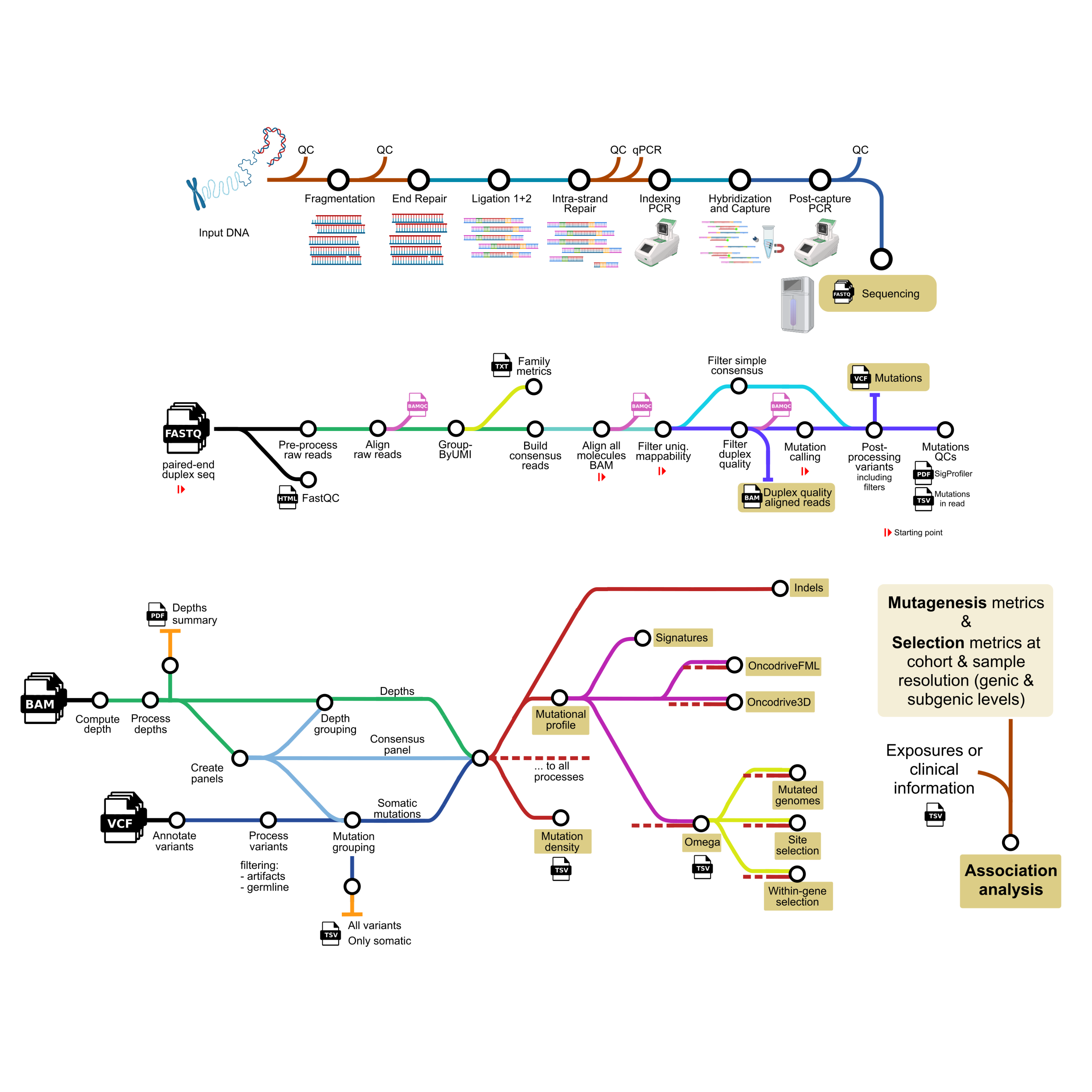
The preparation of libraries for DNA duplex sequencing uniquely tags both ends of each DNA molecule fragment in the sample with a double-stranded barcode, and amplifies by PCR both of its strands. Duplicates arising from each strand are then reunited computationally to form single strand consensus reads and the consensus of both strands arising from the same original fragment are combined to form a double strand (or duplex) consensus read. Nucleotide changes present in both strands of this duplex consensus read must precede the PCR, and are therefore not amplification or sequencing errors, but likely real mutations. The construction of a duplex consensus read from PCR duplicates to detect somatic mutations present in one or a few such consensus DNA molecules requires a tailored computational pipeline. Furthermore, the analysis of mutagenesis and selection from these somatic mutations requires computational methods capable of dealing with the highly heterogeneous sequencing depth that is characteristic of DNA duplex sequencing. This heterogeneity implies that there is a different likelihood to detect mutations at regions sequenced at different duplex sequencing depth and, furthermore, different accuracy in the estimation of their variant allele frequency (VAF) in the sample. DeepClone covers these three steps: 1) the preparation of libraries for DNA duplex sequencing (Fig. 1a; Supp. Note), 2) the construction of double strand consensus sequences and the identification of somatic mutations, (Fig. 1b; Supp. Note) and 3) the analysis of mutagenesis and selection across samples (Fig. 1c,d; Supp. Note).

Applications
The main outcomes of this protocol are metrics of mutagenesis (such as active mutational signatures and mutation density) and selection obtained across samples and the association of these metrics with their history of exposures. When applied to polyclonal samples from in vitro or in vivo models exposed to known or suspected carcinogens, human samples obtained from individuals with different history of exposures, or before and after a potentially life-changing exposure (e.g., chemotherapy treatment, smoking cessation) the protocol can reveal which of these external agents act as mutagens or promoters of pre-existing mutated somatic cells. It can thus be used as a test of the mutagenic22 or clonal promoting effect of any agent (Lopez-Bigas et al., under review). We recently demonstrated the application of this protocol to identify the associations of biological sex with the magnitude of positive selection on truncating mutations of three genes and of a history of smoking with the presence of activating mutations in the TERT promoter across normal urothelial samples23. Other recent articles have reported its use in the investigation of mutagenesis and selection in blood20, buccal epithelium20,29, or sperm27, or across several tissues in autopsies26.
 
We can envision that such a rapid test can be implemented using minimally invasive sampling (e.g., buccal swabs, blood, urine) to monitor specific population strata at higher risk of certain types of cancer, such as head and neck, esophageal or bladder carcinomas. DeepClone can also be applied to the study of subclonal evolution in tumors, in particular, in face of changing selective pressures, such as the exposure to an anti-cancer therapy36. Furthermore, it can be applied to the study of somatic mosaicism associated with cancer37 or other diseases38, or to understand the potential contribution of somatic mutations and clonal expansions to the aging soma39,40.

The systematic application of the protocol to samples of the same tissue probing the mutations in a set of genes under positive selection can also be applied to the problem of saturation mutagenesis (understood here as the assessment of the potential functional impact of all possible mutations in a gene, especially in tumorigenesis). It is predicated on the idea that protein affecting mutations detected in a polyclonal sample reflect multiple expanded clones, which can be regarded as natural experiments revealing which mutations are under positive selection in the tissue in question. In theory, if a sufficiently large number of clones is interrogated (e.g., the cumulative depth resulting from pooling several samples), all mutations under positive selection will appear mutated over the expectation, unlike neutral or deleterious mutations. Two recent articles have demonstrated the power of this approach to build high resolution saturation mutagenesis maps in genes frequently mutated in the bladder urothelium, blood and the buccal epithelium20,23. 

Comparison to other methods 
We briefly compare three similar protocols, DuplexSeq18,25, Targeted NanoSeq20 and UDSeq21 with DeepClone (Supp. Table 1). All four use similar DNA duplex library preparation approaches that exploit the capabilities to uniquely tag DNA fragments in a sample using molecular barcodes (Supp. Table 1). 

DuplexSeq, the first duplex sequencing protocol developed more than a decade ago18,25,28, was based on in house duplex adaptors and originally employed sonication for DNA fragmentation. Sonication, shown to introduce a high number of sequencing artifacts, was later replaced with enzymatic fragmentation, to build a protocol that was commercialized by TwinStrand Biosciences. Recently, Targeted NanoSeq, which followed its untargeted version19, was developed on the basis of DuplexSeq by specifically blocking the repair of DNA fragments through the addition of ddBTPs. This way, the reduced error rate resulting from preventing the ligation of fragments with single-strand nicks, is obtained at the expense of reducing duplex depth and, as a consequence, the sensitivity to identify somatic mutations. Several newer duplex sequencing approaches (UDSeq, and DeepClone) are based on the original SaferSeqS41. DeepClone, however, introduces specific variations to obtain DNA blunt ends in fragmentation and to reduce the number of DNA bases damaged before ligation, while maintaining a number of ligated DNA molecules that is enough to obtain DNA duplex depth per sample above 3,000x (see description below). As explained above, Targeted NanoSeq differs from the other four in lacking a step of DNA end repair, which results in a smaller error rate (<5x10-9 compared to ~10-8 of DeepClone) (Extended Data Fig. 1; Supp. Note). 

Three of the protocols –UDseq, NanoSeq and DeepClone– provide similar computational pipelines to identify the somatic mutations from the DNA duplex sequencing data. DupCaller (UDseq) models the sample-specific error profiles resulting in a slightly more sensitive variant calling compared to NanoSeq21. Only DeepClone includes a computational pipeline that provides an ecosystem of tools to systematically analyze mutagenesis and selection across probed samples (deepCSA). This pipeline endows the user with the capability to run this ecosystem of tools to automatically compute a variety of outcomes, including the mutational signatures active across samples and the magnitude of positive selection on the mutations of different genes in each sample. More importantly, deepCSA furnishes an important number of quality control metrics of these outputs that allow the researcher to steer the analyses depending on their question and the results of intermediate steps (Extended Data Fig. 2-7). For example, deepCSA provides comparisons between the density of non-protein affecting mutations in every gene and the distribution observed across all genes, thus allowing the user to spot genes with extremely high or low values, which could be excluded from the calculation of positive selection with omega. We recommend that the first run of deepCSA in a cohort of samples be used primarily for quality control and not to directly obtain biologically meaningful results (see the Procedure section and Supp. Note). 
 
DeepUMIcaller, the computational pipeline dedicated to identify somatic mutations in the DeepClone protocol can be easily coupled to DNA duplex data generated from different duplex library preparations (this was done in the original article presenting deepUMIcaller23). Similarly, deepCSA can be used on somatic mutations identified by other DNA duplex sequencing protocols and variant calling pipelines. This guarantees the flexibility needed to select different experimental approaches depending on specific research questions (see next section) at the convenience of the user. Both computational pipelines have been developed in Nextflow42, increasing their portability and scalability.

Experimental design
The experimental design –starting DNA amount, specific DNA duplex library preparation (e.g., out of the four presented above), panel of genes to target, number of samples– needs to be guided by the research question (Supp. Note). Below, we describe the rationale to select the approach that is best suited for some typical research questions that can be tackled using DNA duplex sequencing.

If the aim of the experiment is to study mutagenesis (e.g., the mutational processes active in a tissue and the mutation density), the key element is to sample a representative set of all possible tri-nucleotides, as well as enough mutations to identify even mutational signatures with relatively low activity across samples. This depends on the number of sampled sites, which is determined, ultimately by the product of the selected genomic region and the average depth of sequencing. As a result, if the region of the gene targeted for capture is sufficiently large, high sequencing depth is not required. All four protocols described in the previous section are well suited for this purpose.

When the researcher’s goal includes the discovery of genes under positive selection in a tissue, the genomic region to target becomes more important, and so does the duplex sequencing depth. In this case, the panel only needs to include genic regions that may be under selection (relevant genes or non-coding regions with known regulatory function, such as the TERT promoter). Since the cost of sequencing the whole exome at sufficient depth across samples can scale very quickly, it is recommendable to target only the exons of a set of genes with reasonable probability to be under selection in the tissue in question, such as genes that drive tumors that arise from it, and/or genes already observed under selection in previous studies. In order to discover genes under positive selection, one requires enough statistical power to run computational driver discovery methods (such as those included in deepCSA; Supp. Note). This requires the identification of a sufficient number of protein and non-protein affecting mutations across samples. The latter critical requirement may be difficult to meet for short genes, with relatively few synonymous sites, such as TP53. If the duplex sequencing depth obtained per sample is not very high (e.g., below 1,000x), the experiment will require more samples to reach the minimum required number of mutations to run driver discovery methods. The same reasoning applies if the aim of the experiment is natural saturation mutagenesis (see above).

Finally, probing the association between the exposure to intrinsic (e.g., those associated with age or sex) or exogenous factors (e.g., tobacco smoking, alcohol drinking, or cytotoxic drugs) and the clonal landscape of a tissue requires to accurately infer the magnitude of positive selection shaping the mutational landscape of each gene of interest in each sample23. This type of analysis requires the interrogation of an even more reduced set of genes (only those with positive selection in the tissue in question, as others would be non-informative) and higher duplex depth per sample. Reaching the required depth per sample is difficult for Targeted NanoSeq, due to its DNA duplex library protocol, and for UDSeq, optimized for very low starting DNA quantities21. Overcoming this limitation to gain sufficient statistical power to do this analysis at scale requires either to prepare multiple duplex libraries using the DeepClone protocol, or the use of a more efficient and not limited DNA duplex library preparation (Supp. Note). We have demonstrated that both solutions work with DeepClone23.

Sample requirements
It is critical to extract and manipulate the genomic DNA (gDNA) of interest in non-strand-denaturing conditions. We recommend using the DNeasy Blood & Tissue kit (Qiagen, cat. no. 69506) and if low DNA yield is expected, the QIAmp DNA micro kit (Qiagen, cat. no. 56304) is also suitable. The gDNA can be resuspended in a low-EDTA buffer such as low TE (10 mM Tris-Cl, 0.1mM EDTA, pH 8.0) or AE buffer (10 mM Tris-Cl, 0.5mM EDTA, pH 9.0). We recommend eluting the gDNA in a volume that will yield a suitable concentration range for optimal sample preparation. Upon quantification with fluorescence-based methods, such as Qubit, the desired gDNA input should be in a volume equal or less than 26 μL. If the gDNA is too diluted, bead-based or column-based methods are recommended for reconcentration. Evaporating methods (such as speed-vac) should be avoided to prevent salt concentration that can impair downstream steps. gDNA integrity should be assessed with a Genomic DNA ScreenTape Assay and run on an Agilent TapeStation 4200 or similar right before starting the DNA duplex library protocol, to account for any DNA integrity variations during sample shipping and/or storage. This protocol has been optimized for using high-molecular weight gDNA as input (DIN value above 6). Starting with lower-quality DNA is possible but the fragmentation step needs to be tailored to avoid overfragmentation. Certain damage to the DNA introduced in the process of extraction or storage, or during fragmentation (e.g., single-stranded ends) could lead to a change in both strands in the DNA molecule as a consequence of the end repair process, which may then be wrongly identified as a somatic mutation. These changes of nucleotide in both strands that precede the ligation to duplex sequencing barcodes and are not due to mutational processes active in the tissue are known as pseudo-duplex nucleotide changes.

DNA fragmentation
Obtaining an optimal size distribution of fragments of gDNA is critical for library preparation and sequencing efficiency. To avoid single-stranded hanging ends in the fragmentation (see previous section), we chose to do an enzymatic fragmentation of the gDNA using the NEB UltraShear. The incubation time depends on sample characteristics (quantity, integrity of the starting DNA, elution buffer). Therefore a kinetics test is recommended to decide the optimal fragmentation conditions and maximize the number of DNA fragments with appropriate size for short-read NGS sequencing. The efficiency assessment of fragmentation can be performed by High Sensitivity DNA ScreenTape Assay and run on an Agilent TapeStation 4200 or similar, measuring the region ranging between 50 and 650 bp. The protocol has been designed to achieve optimal fragmentation status across samples being processed in parallel in one DNA duplex library preparation (see Figure 2 for an example case). However, the incubation step can be extended for specific samples in the batch, if needed. To decide the necessary sample-specific adjustment, all samples are kept on ice while running the High Sensitivity DNA ScreenTape Assay, and we recommend this time to be kept to a minimum, to prevent undesired overfragmentation.

Ligation
Most duplex sequencing methods use adapters with double-stranded molecular barcodes. Here we use a two step ligation method commercially available, which uses adapters with 8 bp molecular barcodes, without T overhangs. These are first ligated on the 3’ end of the insert, and in the second ligation the other adapter strand is added by gap filling to generate the double-stranded molecular barcodes. 

Intra-strand repair
Damaged bases are susceptible to being fixed as mutations during the PCR amplification, and therefore detected as false-positive mutations. Consequently, the protocol incorporates a repair step before the indexing PCR to remove 8-oxo-7,8-dihydroguanine (8-oxoG) and uracil resulting from deaminated cytosines.

Quantification of unique ligated DNA fragments with qPCR
This technique allows us to specifically quantify the number of unique DNA fragments that have been successfully ligated with the duplex adapters. This number depends on the input DNA and the efficiency of the duplex library preparation steps, especially the ligation. Basing the calculation of required sequencing reads on the number of ligated molecules estimated in this step avoids oversequencing (too many PCR duplicates sequenced per original DNA fragment) or undersequencing (too few sequencing reads to form consensus duplex reads). However, if the efficiency of the duplex library preparation is constant, the sequencing reads can also be directly calculated based on the input DNA for each sample (Supp. Note). 

Increasing duplex depth
The described protocol has a limitation of 250 ng of starting material. This input may not be enough to reach the desired duplex depth. In the cases where more starting material is available, it is possible to start with more than one DNA duplex library per sample. After the libraries are amplified and uniquely tagged in the indexing PCR with Unique Dual Index (UDI) tags, libraries prepared from the same sample can be multiplexed for hybridization and capture with the desired targeted panel. We highly recommend multiplexing libraries that have a similar number of unique DNA fragments by qPCR and similar library sizes determined by TapeStation, since after pooling the different libraries they will be processed as a unique sample and will be sequenced together. In addition, we recommend only multiplexing up to 2 libraries from the same gDNA of origin.

Hybridization and capture
The minimum input of the amplified library recommended to go into the hybridization reaction is 100 ng. However, we recommend starting with 2-3 μg and do not exceed 6 μg as this could affect the capture’s performance, as per manufacturer’s instructions. Further recommendations regarding hybridization annealing time and number of post-capture PCR cycles are described in the procedure, although it is highly recommended to test those variables depending on the panel used to capture the target regions of interest. For panels <100kb we recommend two consecutive rounds of hybridization capture, as previously described25, to obtain sufficient on-target reads. 

Sequencing
The required sequencing output is estimated on the basis of the amount of unique DNA ligated fragments, calculated by qPCR (see above), the size of the capture panel, how many PCR duplicates are required on average to produce one consensus duplex read, and the efficiency of the hybridization capture (Supp. Note). As mentioned above, if too few sequencing reads are obtained, one may end up without enough PCR duplicates to form the expected number of duplex consensus reads (ideally, one per ligated DNA fragment). In this case the library is undersequenced, and this problem can be solved by requesting more sequencing reads. On the other hand, if too many sequencing reads are obtained, this will result in more PCR copies per ligated DNA fragment but duplex depth will not increase since the number of possible duplex consensus reads is limited. This problem, known as oversequencing, implies that more resources than necessary have been spent in sequencing the library in question. We have carried out the sequencing of DNA duplex libraries on Illumina NovaSeq 6000 and Illumina NovaSeq X instruments23.

Building duplex consensus sequences
The deepUMIcaller pipeline receives the reads produced by the sequencer from a library and outputs a list of the somatic mutations present in it. It can be run serially or in parallel (see Supp. Note for how this is achieved in each step of the pipeline). Parallel running is recommended in the case of ultradeep sequencing libraries captured with large sequencing panels (e.g. more than 100 genes).

The deepUMIcaller pipeline requires demultiplexed pairs of FASTQ files from each sample as input. If this is split in multiple pairs of FASTQs (e.g., if the sample has been sequenced on multiple lanes), the pipeline will run in parallel mode, thus speeding up the first steps of raw read processing and alignment. After extracting the duplex tags, we recommend to set an automatic clipping of the first 10 bps of the reads to reduce potential artifacts usually seen at the beginning of the reads. Once the sequencing reads are aligned, the pipeline proceeds to build single and double strand consensus using the fgbio suite of tools, and calibrated duplex quality thresholds (see Supp. Note). This process can be executed separately by chromosome to reduce the execution time.
As a final step of the duplex building process, deepUMIcaller writes the BAM files with single strand and duplex consensus reads mapped to the reference genome passing an unambiguity threshold (AS-XS > 50; Supp. Note). This file contains the maximum number of original DNA fragments that are available to identify somatic mutations. If multiple libraries have been prepared from the same sample (see Increasing duplex depth section) these can be merged at this step in order to proceed to the variant calling. This merging is implemented in deepUMIcaller and it can be triggered by assigning the same name in the parent_dna column of the input file (see: https://github.com/bbglab/deepUMIcaller/tree/master/docs for more information).

Variant calling
The BAM files containing all unique molecules generated in the consensus building steps can next be filtered to keep only duplex consensus reads with at least 2 copies supporting each of its single strand consensus to proceed to the variant calling. We use VarDictJava in pileup mode for calling all the potential genetic variants and this process is followed by the application of successive filters based on different criteria. These filters add flags to the FILTER column of the VCF file, which can then be used to discard specific sets of potential artifacts (see Supp. Note). These filters include genomic regions of low complexity, problematic mappability, polymorphic positions or genomic sites with recurrent sequencing errors, which are applied using a set of BED and mask files20.

Variant allele frequency calculation
The quotient between the number of duplex reads with a mutation and the total number of duplex reads covering the genomic position yields the variant allele frequency (VAF) of the mutation on DNA duplex reads, or duplex VAF. Despite calling mutations only if they are supported by both single strand consensus in a duplex consensus read, we can leverage the information from the rest of unique molecules sequenced to refine (with more reference and alternate reads) the calculation of the variant allele frequency of a mutation. Thus, we compute a second VAF value taking into account all unique molecules (including those that do not form a duplex consensus), which we call the all molecules VAF. We compute a third VAF value using exclusively the unique molecules that do not form a duplex consensus. This third metric is called no duplex VAF. The three values are, of course, highly correlated. The all molecules or no duplex VAF metrics always include more reads and are therefore preferred to avoid low-depth related artifacts (Supp. Note).

Quality controls
DeepUMIcaller generates multiple QCs that allow evaluation of key library preparation and sequencing parameters. These include the rate of duplicates of original DNA fragments, the percentage of raw sequencing and duplex consensus reads on target, the overall sequencing depth, and others. In addition, a final quality check for each sample consists of plotting the distribution of the mutations along the positions of the reads to identify potential enrichment on the first bases due to DNA damaged bases at read ends (Figure 4). If the increase of variants remains despite clipping the first 10 bases of reads, the clipping should be extended further. 

DeepUMIcaller additional run modes
Several additional parameters can be tuned according to the user's preferences, and there are also multiple possible starting points depending on the input data available. For more information on all possibilities, see the documentation at the GitHub repository: github.com/bbglab/deepUMIcaller/blob/dev/docs. Only starting from the mapping step allows the generation of all QC metrics required for downstream compilation.

Integrated duplex metrics
These scripts compile the QCs from the library preparation with the results of data processing to allow quality assessment of the duplex data generated. The value of these metrics (Supp. Table 2) increases with the availability of more samples so it is critical to compile all the runs together in the templates provided. All the code required for the computation of this and other metrics is available here: https://github.com/bbglab/wetdry-metrics and see Supplementary Note for more information.

Assemble a cohort
For the applications of DNA duplex sequencing described above, ideally, one would assemble a cohort of polyclonal samples with enough DNA to obtain a duplex sequencing depth that is enough to answer the desired research questions. At least 250 ng of DNA are needed to achieve a mean duplex depth of ~3,000x; if deeper DNA duplex sequencing is required, more input DNA should be used. If the aim of the project is to understand the effect of internal or endogenous exposures on mutagenesis and selection in a cohort, samples with different exposures in numbers sufficient to achieve the necessary statistical power, given the expected effect sizes, must be included in the cohort. Groups of samples (for example depending on exposures) can be defined when executing deepCSA, so that analyses are run on each sample, on each group of samples, and across all samples.

Select mutations in well-covered regions across samples
To avoid biases introduced by areas with different coverage across samples, only mutations in well-covered regions across samples are selected for analyses (at least ~200x, but dependent on average depth of the cohort). This is one of the first steps of deepCSA, which generates a file with the selected genomic regions that we refer to as the consensus panel. To carry out this step, the user needs to provide both a VCF file with mutations and a BAM file with the duplex quality reads for each sample. Both files can be directly obtained from the output of deepUMIcaller. If another computational pipeline is used to identify mutations, these files need to be extracted from their outputs and fed to deepCSA. 

Annotate and filter mutations
All the mutations provided to deepCSA are annotated using Ensembl VEP and are assigned a consequence type based on their impact on the corresponding MANE transcripts. The sequencing coverage information is also added for each mutation, as well as the flags warning about potentially artifactual mutations (cohort n-rich, repetitive, potential SNP23). After all the preprocessing steps, the pipeline applies the desired set of filters (filters_criteria, filter_criteria_somatic; Supp. Note). This includes VAF thresholds to discard rare or private germline variants and flags generated by prior steps of the pipeline. These filtered mutations, together with the depths per position and the consensus panel, constitute the main inputs for all downstream analysis of mutagenesis and selection implemented by deepCSA. 

Analysis of mutagenesis
The basic mutagenesis metrics implemented within deepCSA are mutation densities and mutational profiles. The mutation density of a gene in a sample (or across groups of samples) is computed by dividing the total number of somatic mutations with a given consequence (e.g., protein-affecting or non-protein-affecting mutations) that were sequenced in the gene. This total number of sites is calculated as the product of the total number of sites with potentially the same consequence type in the gene, multiplied by the number of times each of them is covered by a duplex consensus read (in Mbps). The mutational profile computed by deepCSA is the classical tri-nucleotide context single base substitution (SBS) profile of 96 channels, resulting from the quotient of the number of tri-nucleotide changes observed by the number of times the given tri-nucleotide was sequenced and re-scaled to the whole genome trinucleotide counts (https://github.com/bbglab/deepCSA/blob/main/docs/output.md). DeepCSA uses the SBS mutational profile across samples to identify the mutational signatures active in the cohort through HDP33 and SigProfilerAssignment15, on the basis of a reference set of signatures provided by the user (e.g., the COSMIC43 reference). 

Selection analyses
The analysis of selection requires tools specifically adapted for duplex sequencing data. To this end, we developed a new method to compute dN/dS-based positive selection signals called omega (ref.23, Supp. Note) and we adapted OncodriveFML34 and Oncodrive3D35 to use position specific weights that ensure a proper correction for the uneven depth per site in the calculation of their background models. The ultradeep sequencing of multiple polyclonal samples results in hundreds of mutations for some genes enabling the possibility of computing selection metrics at subgenic or even site resolution. The omega method can compute the selection signals for each exon, known protein domains or other custom regions. Additionally, we provide estimates for site specific selection, particularly useful for quantifying selection in known hotspots and for natural saturation mutagenesis, where we can estimate the effect of every possible mutation in a given gene. All these measurements of mutagenesis and selection define the mutational and clonal landscape of the tissue/cohort of interest.

Interindividual variability and associations with clinical variables
DeepCSA also includes a regression-based approach to test the association between the exposure to endogenous or exogenous factors, or any other clinical data, and the clonal landscape of samples. This can serve as a first pass exploration of potential relationships (Supp. Note). For a more fine-tuned analysis, a more comprehensive module of data exploration and regressions can be used (https://github.com/bbglab/bbgregressions). This part of the pipeline is, of course, dependent on the user providing metadata of the samples that contain relevant exposures to test (Fig. 1d). 

Fragmentation and cleanup

1h 30m

Ensure that the NEBNext UltraShear Reaction Buffer is completely thawed and quickly vortex to mix. Place on ice until use.

Vortex the NEBNext UltraShear for 5–10 s prior to use and place on ice.
CRITICAL STEP: It is important to vortex the enzyme mix prior to use for optimal performance.

Add the following components to a 0.2 mL thin wall PCR tube on ice:

CRITICAL STEP: If processing more than one sample, make a mastermix with 10% overage.

Vortex the reaction for 5–10 s and briefly spin in a microcentrifuge.

In a thermal cycler, preheated and with the heated lid set to 75 °C, run the following program:

Transfer samples immediately to ice, and assess fragment size in TapeStation using 1 μL diluted 1:5 in sterile water and following manufacturers instructions.

If the percentage of DNA fragments in the 50-650bp region assessed by TapeStation is below 30%, add extra time on the Fragmentation program and check again.

Once samples have reached this 30% threshold of DNA fragments within 50-650bp, proceed to the next step.

For easier handling of the sample and faster collection of the beads to the magnet, it is recommended to dilute the sample with sterile water. Add 6 μL nuclease-free water (or up to 50 μL) to the sample.

Thoroughly resuspend AMPure XP beads before use, then add 90 μL of AMPure beads (1.8X volume) to each tube and pipette 10 times to thoroughly mix.

Incubate the samples at room temperature for 10 min.

Place the samples on a magnet and wait for the liquid to clear completely or at least for 2 min.

Remove and discard the cleared supernatant making sure not to remove any beads.

Keeping the samples on the magnet, add 160 μL of 80% ethanol and incubate for 30 s.

Remove and discard the supernatant.

Repeat steps 14 and 15 for a total of 2 washes.

Use a P10 pipette tip to remove any residual ethanol.

Dry the beads at room temperature for 1–3 min.

Remove the samples from the magnet, then add 52 μL of Buffer EB and resuspend beads fully.

Allow the samples to incubate at room temperature for 5 min to elute DNA off the beads.

Place the samples on a magnet and wait for the beads to be cleared from the liquid (approximately 1–2 min).

Carefully transfer 52 μL of the cleared liquid containing the eluted DNA into a new well.

Quantify 1 μL the fragmented product with a Qubit HS assay and assess its size distribution using 1 μL in an Agilent TapeStation 4200 or similar. Fragmented products at this point should be around 250-350 bp. Proceed to the next step with the remaining 50 μL.

End repair and cleanup

For each sample, make the following End Repair Master Mix:

CRITICAL STEP: If there is precipitate in the End Repair Buffer, vortex until the precipitate becomes clear in solution.
CRITICAL STEP: The resulting Master Mix is viscous and requires careful pipetting.

Pulse-vortex the master mix for 10 s, then briefly centrifuge. Keep the master mix on ice.

Add 9 μL of End Repair Master Mix to each well. Using a pipette set to 40 μL, pipette 10 times to mix.

In a thermal cycler, with the heated lid set to OFF, or to 40 °C, run the following program:

While the end repair program runs, make the Ligation 1 Master Mix in preparation for the Post-End Repair cleanup steps.

Pulse vortex the master mix for 10 s, then briefly centrifuge. Keep the master mix on ice until ready to use.

After the End Repair program reaches 4 °C, proceed immediately to the bead cleanup.
CRITICAL STEP: Before starting cleanup, make sure the Ligation 1 Master Mix has already been prepared.

Thoroughly resuspend AMPure XP beads before use, then add 147.5 μL of AMPure beads (2.5X volume) to each well and pipette 10 times to thoroughly mix.

Incubate the samples at room temperature for 10 min.

Place the samples on a magnet and wait for the liquid to clear completely or at least for 2 min.

Remove and discard the cleared supernatant making sure not to remove any beads.

Keeping the samples on the magnet, add 160 μL of 80% ethanol and incubate for 30 s.

Remove and discard the supernatant.

Use a P10 pipette tip to remove any residual ethanol.

Dry the beads at room temperature for 1–3 min.

Ligation 1

30m

Remove the samples from the magnet, then add 30 μL Ligation 1 Master Mix.

Pipette mix a minimum of 10 times.
CRITICAL STEP: Make sure the samples are thoroughly mixed and that the beads are fully resuspended before proceeding.

In a thermal cycler, preheated and with the heated lid set to 70 °C, run the following program:

PAUSE POINT: The samples can temporarily remain at 4 °C (no more than 2 hours). It is normal for beads to settle during this reaction.

Ligation 2 and cleanup

For each sample, prepare the Ligation 2 Master Mix.

Pulse-vortex the master mix for 10 s, then briefly centrifuge. Keep the master mix on ice until ready to use.

Add 10 μL of the Ligation 2 Master Mix to each well.

Using a pipette set to 35 μL, pipette 10 times to mix.
CRITICAL STEP: Make sure the samples are thoroughly mixed and that the beads are fully resuspended before proceeding.

In a thermal cycler, preheated and with the heated lid set to 70 °C, run the following program:

Add 100 μL of PEG/NaCl (2.5X volume) to each well, then pipette 10 times to mix.

Incubate the samples at room temperature for 10 min.

Place the samples on a magnet and wait for the liquid to clear completely or at least for 2 min.

Keeping the samples on the magnet, add 160 μL of 80% ethanol and incubate for 30 s.

Remove and discard the supernatant.

Repeat steps 49 and 50 for a total of 2 washes.

Use a P10 pipette tip to remove any residual ethanol.

Dry the beads at room temperature for 1–3 min.

Remove the samples from the magnet, then add 25 μL of Buffer EB and resuspend beads.

Allow the samples to incubate at room temperature for 5 min to elute DNA off the beads.

Place the samples on the magnet and wait for the beads to be cleared from the liquid (approximately 1–2 min).

Carefully transfer 25 μL of the cleared liquid containing the eluted DNA into a new tube.
PAUSE POINT: Samples can be stored at –20 °C overnight.

Intra-strand repair and cleanup

1h 30m

For each sample, prepare the Intra-strand repair Master Mix:

Pulse-vortex the master mix for 10 s, then briefly centrifuge. Keep the master mix on ice until ready to use.

Add 5 μL of the Intra-strand repair Master Mix to each sample.

Using a pipette set to 25 μL, pipette 10 times to mix.

If necessary, briefly centrifuge to collect contents to the bottom of the wells.

In a thermal cycler, preheated and with the heated lid set to 40 °C, run the following program:

Once incubation is over, add 20 μL of nuclease-free water to each reaction and proceed to the bead cleanup.

Thoroughly resuspend AMPure XP beads before use, then add 45 μL (0.9X volume) of Agencourt AMPure XP beads to each sample.

After adding the beads, mix thoroughly and incubate for 10 min.

Place the samples on a magnet until the supernatant is clear (2–5 min).

Remove supernatant without disturbing the beads.

While keeping the samples on the magnet, add 125 μL of 80% ethanol, then incubate for 30 s.

Remove and discard the supernatant.

Repeat steps 69 and 70 for a total of 2 washes.

Use a P10 pipette tip to remove any residual ethanol.

Allow the beads to air dry for 1–3 min. Do not over-dry the beads.

Remove the samples from the magnet and elute in 23 μL of Buffer EB. Mix thoroughly.

Incubate for 5 min at room temperature.

Place the samples on a magnet until the supernatant is clear (1–2 min).

Transfer 23 μL of eluate to a fresh tube making sure that no beads are carried over.

Quantify 1 μL the product with a Qubit HS assay and assess its size distribution using 1 μL in an Agilent TapeStation 4200 or similar. Fragmented products at this point should be around 350-450 bp. Proceed to the next step (Indexing PCR) with the remaining 20 μL.

Quantification of unique ligated DNA fragments with qPCR

Taking into account the previous quantification, dilute samples accordingly by doing serial dilutions in nuclease-free water, knowing that the six standards are in the range of 5.5 – 0.000055 pg/μL. The recommendation would be to dilute samples at least to around ~1 pg/μL and test two different dilutions. This quantification is not strictly required before proceeding to the next step (Indexing PCR). It is performed to inform about the number of ligated molecules to properly allocate raw sequencing reads when the duplex library is ready for sequencing (see Supp. Note).

For each reaction (which will be in triplicate), make the following mastermix adding an overage of 2 reactions:

Set up triplicate 10 μL qPCR reactions (8 μL master mix, 2 μL sample/standard) in a 384 well plate. Add also a negative control with nuclease-free water.
PAUSE POINT: Samples can be stored at −20 °C overnight.

Run samples on a qPCR thermocycler and run the following programme:

Indexing PCR and cleanup

1h 30m

Add 5 μL of xGen UDI Primer Pairs to each well.
CRITICAL STEP: Sample index barcodes are introduced during PCR; double-check that a unique primer pair is used for each sample.

Add 25 μL of xGen 2x HiFi PCR Mix to each well, then pipette 10 times to mix.

Then briefly centrifuge to recover any volume from the walls into the bottom of the wells.

In a thermal cycler, preheated and with the heated lid set to 105 °C, run the following program:

Thoroughly resuspend AMPure XP beads before use, then add 45 μL of AMPure beads (0.9X ratio), to each well, then pipette 10 times to thoroughly mix.

Incubate the samples at room temperature for 5 min.

Place the samples on a magnet and wait for the liquid to clear completely or at least for 2 min.

Remove and discard the cleared supernatant; make sure not to remove any beads.

Keeping the samples on the magnet, add 160 μL of 80% ethanol, then incubate for 30 s.

Remove and discard the supernatant.

Repeat steps 91 and 92 for a total of 2 washes.

Use a P10 pipette tip to remove any residual ethanol.

Dry the beads at room temperature for 1–3 min.

Remove the samples from the magnet, then add 32 μL of Buffer EB. Gently vortex (use 70% vortex capacity) to resuspend beads.

Allow the samples to incubate at room temperature for 5 min to elute DNA off beads. Then place the samples on a magnet and wait for the liquid to clear completely for 1–2 min.

Carefully transfer 32 μL of eluted DNA into a new tube.

Quantify 1 μL the PCR product with a Qubit HS assay and assess its size distribution using 1 μL in an Agilent TapeStation 4200 or similar. Fragmented products at this point should be around 350-650 bp.

Hybridization

Use half of the Indexing PCR product for capture and keep the other half at -20 ºC as a back up sample. If capture fails, the second half can be used for recapture. If samples are being multiplexed, pool half of each Indexing PCR product combined into a single tube.

Add 7.5 μL of Human Cot DNA.

Add 1.8X volume of AMPure XP beads.

Vortex thoroughly to mix. Adjust the settings to prevent any splashing onto the seal or cap.

Incubate for 10 min at room temperature.

Incubate the samples on the magnet for at least 2 min or until supernatant is clear.

Remove and discard the supernatant. Keeping the samples on the magnet, add 80% ethanol to cover the surface of the beads. Incubate for 30 s without disturbing the beads.

Remove and discard the supernatant, then repeat another ethanol wash for a total of two washes.

Allow the beads to air dry for approximately 3 min.
CRITICAL STEP: Do not over-dry.

Add these components to the tube to make the Hybridization Reaction Mix:

Remove the samples from the magnet and vortex to mix. Ensure that the beads are fully resuspended.

Incubate for 5 min at room temperature.

After incubation, place the samples on a magnet for 5–10 min or until the supernatant is clear.

Transfer 18 μL (or all the volume you are able to recover without taking any beads) of the supernatant to a new well, where the hybridization will occur. Make sure to avoid bead carryover during the transfer process.

Vortex briefly to mix and spin down.

Incubate the samples in a thermal cycler, preheated and with the heated lid set to 100 °C, run the following program:

CRITICAL STEP: The annealing time should be optimized per panel size, for reference, for relatively big panels (>17,000 probes) we recommend doing an overnight annealing (equivalent to a minimum of 16 h incubation).

Streptavidin bead wash

30m

Prepare the following buffer to create a 1X working solution:

Prepare the following Bead Resuspension Mix in a low-bind tube:

Add 50 μL of capture bead-mix per sample to 1.5 mL tube.

Collect the beads on a magnet and remove the supernatant.

Add twice the volume of bead-mix of 1X Bead Wash Buffer to the tube. For example, if 500 μL of bead-mix is being washed, use 1 mL of Bead Wash Buffer.

Remove from the magnet and briefly vortex the beads to resuspend, then spin down.

Collect the beads on a magnet and remove the supernatant.

Repeat steps 120−122 twice more for a total of 3 washes.

Following the last wash, collect the beads on the magnet and remove the supernatant.

Remove from the magnet and resuspend the beads in 17 μL of the Bead Resuspension Mix per reaction. Mix solution thoroughly pipetting until homogenous. If necessary, spin down briefly at low speed to avoid bead pelleting.

Capture

Remove samples from the thermal cycler and stop the Hybridization program. Immediately start the Wash program.
CRITICAL STEP: Before adding the beads to your samples, vortex or pipette mix the washed bead-mix to ensure uniformity.

Spin down the tubes briefly to ensure no sample or condensation is left on the seal or tube cap.

Ensure washed capture beads are homogeneously resuspended immediately before aliquoting.

Add 17 μL of resuspended washed capture beads to each sample at room temperature.

Gently vortex the samples to resuspend the mixture.

Incubate the samples in a thermal cycler, preheated and with the heated lid set to 70 °C, and run the following program:
CRITICAL STEP: Reduce the lid temperature to 70 °C for the Wash program.
CRITICAL STEP: Every 10–12 min, remove the tube from the thermal cycler and gently vortex to ensure the sample is fully resuspended.

At the end of the 45 min, take the sample off the thermal cycler and proceed immediately to Heated washes.

Heated washes

30m

Dilute the following xGen buffers to create 1X working solutions:

CRITICAL STEP: Inspect the xGen 10X Wash Buffer I. If it appears cloudy, warm solution to 65 °C and mix until homogeneous. Allow it to cool to RT after heating. Use all Wash buffers at RT.

Aliquot 110 μL per sample of the 1X Wash Buffer 1 into a separate tube. Heat tubes to 65°C in the thermocycler with the Wash program. The remaining solution should be kept at room temperature.

Aliquot 160 μL each per sample into two tubes (with 160 μL each) of the 1X Stringent Wash Buffer. Heat tubes to 65°C in the thermocycler with the Wash program. 
CRITICAL STEP: The 1X Wash Buffer 1 (110 μL aliquot) and the 1X Stringent Wash Buffer (both aliquots) should be in the 65 °C thermocycler with the Wash program for at least 15 min. We recommend starting this incubation at the same time as the bead capture, so that the buffers will be at the correct temperature when needed.

After capture, spin down and place the samples on a magnet to collect the beads.

Transfer 100 μL of heated Wash Buffer 1 to the sample, then pipette mix 10 times, being careful to minimize bubble formation.

Place the tube on a magnetic rack for 1 min. Remove the supernatant.

Remove the tube from the magnet and add 150 μL of heated Stringent Wash Buffer to the sample. Pipette mix 10 times, being careful to not introduce bubbles.

Incubate in the thermocycler at 65 °C for 5 min.

Place the tube on a magnetic rack for 1 min. Remove the supernatant.

Place the tube on a magnetic rack for 1 min. Remove the supernatant. Use a P10 to remove any residual liquid.

Incubate in the thermocycler at 65 °C for 5 min.

Place the tube on a magnetic rack for 1 min. Remove the supernatant. Use a P10 to remove any residual liquid.

Room temperature washes

30m

Add 150 μL of Wash Buffer 1 equilibrated to room temperature.

Vortex thoroughly until fully resuspended.

Incubate for 2 min while alternating between vortexing for 30 s and resting for 30 s, to ensure the mixture remains homogenous.

At the end of the incubation, briefly centrifuge the tube.

Place on the magnet for 1 min.

Remove the supernatant. Add 150 μL of Wash Buffer 2.

Vortex thoroughly until fully resuspended.

Incubate for 2 min while alternating between vortexing for 30 s and resting for 30 s, to ensure the mixture remains homogenous.

At the end of the incubation, briefly centrifuge the tube.

Place on the magnet for 1 min.

Remove the supernatant. Add 150 μL of Wash Buffer 3.

Vortex thoroughly until fully resuspended.

Incubate for 2 min while alternating between vortexing for 30 s and resting for 30 s, to ensure the mixture remains homogenous.

At the end of the incubation, briefly centrifuge the tube.

Place the sample tube on the magnet for 1 min.

Remove and discard the supernatant.

Use a P10 to remove any residual liquid.

Add 20 μL of Nuclease-Free Water to each capture.

Pipette mix 10 times to resuspend any beads stuck to the side of the tube.

Post-capture PCR and cleanup

In a tube, prepare the Amplification Reaction Mix:

Add 30 μL of Amplification Master Mix to each sample for a final reaction volume of 50 μL.

Then gently vortex to thoroughly mix the reaction.

If necessary, briefly centrifuge to collect contents to the bottom of the wells.

Place the samples in a thermal cycler, and run the following program with the lid temperature set to 105 °C:

CRITICAL STEP: The number of PCR cycles should be optimized per panel size. For reference for a panel size of >17,000 probes we recommend to start with 13 cycles of amplification.

Add 45 μL of AMPure beads (0.9X ratio), to each sample, then pipette 10 times to thoroughly mix.

Incubate the samples at room temperature for 5 min.

Place the samples on a magnet and wait for the liquid to clear completely or at least for 2 min.

Remove and discard the cleared supernatant, and make sure not to remove any beads.

Keeping the samples on the magnet, add 160 μL of 80% ethanol, then incubate for 30 s.

Remove and discard the supernatant.

Repeat steps 173 and 174 for a total of 2 washes.

Use a P10 pipette tip to remove any residual ethanol.

Dry the beads at room temperature for 1–3 min.

Remove the samples from the magnet, then add 22 μL of Buffer EB.

Gently vortex (use 70% vortex capacity) to resuspend beads.

Allow the samples to incubate at room temperature for 5 min to elute DNA off beads. Then place the samples on a magnet and wait for the liquid to clear completely for 1–2 min.

Carefully transfer 22 μL of eluted DNA into a new tube.

Quantify 1 μL the PCR product with a Qubit HS assay and assess its size distribution using 1 μL in an Agilent TapeStation 4200 or similar. Final libraries should yield >15-20 ng/μL and fragment distribution should be between 350-650 bp. At this point libraries are ready for sequencing in an Illumina platform or equivalent. 

Sequencing data processing: consensus building, QCs and variant calling

The reference genome needs to be uncompressed and indexed, which can be achieved using the following commands:
gunzip <genome>.fa.gz
	bwa index <genome>.fa
	samtools faidx <genome>.fa
	gatk-launch CreateSequenceDictionary -R <genome>.fa

Clone the GitHub repository: bbglab/deepUMIcaller and move inside the directory.
git clone https://github.com/bbglab/deepUMIcaller.git
cd deepUMIcaller

Generate the low complexity file from the RepeatMasker information. The script accepts RepeatMasker .out files (compressed or uncompressed) and generates a BED format file containing filtered repetitive regions suitable for variant calling exclusion. This can be done for any species.

python assets/generate_low_complex_rep_bed.py hg38.fa.out.gz 
low_complexity_regions.bed

Prepare your input.csv file. For each sample provide: sample (sample name), fastq_1, fastq_2 and read_structure. The sample name can be composed of alphanumerical characters, ‘-’ and ‘_’. The read structure has to follow the fgbio guidelines (https://github.com/fulcrumgenomics/fgbio/wiki/Read-Structures). See example of a file below:
sample,fastq_1,fastq_2,read_structure
sample1,sample1_R1.fastq.gz,sample1_R2.fastq.gz,8M1S+T 8M1S+T
sample2,sample2_R1.fastq.gz,sample2_R2.fastq.gz,8M1S+T 8M1S+T
sample3,sample3_R1.fastq.gz,sample3_R2.fastq.gz,8M1S+T 8M1S+T
…

Create a params.deepUMIcaller.yml file with all the customized parameters. Special attention should be given to the required input parameters, the desired outputs and duplex quality standards. Full documentation of the parameters can be found in the extended protocol and in the deepUMIcaller repository.
input 			  : <input.csv>
ref_fasta 			  : <reference Fasta file>
targetsfile             : <BED: targeted regions>
filter_min_reads_duplex : 4 2 2
perform_qcs             : true

If available, add the BED files required for filtering the mutations in the post-processing steps to the params.deepUMIcaller.yml file.
low_complex_file        : null
low_mappability_file    : null
nanoseq_snp_file        : null
nanoseq_noise_file      : null

You should now proceed to launch deepUMIcaller via the following Nextflow command:
nextflow run bbglab/deepUMIcaller \
  -profile singularity \
  -c executor.config \
  -params-file params.deepUMIcaller.yml

Sequencing metrics compilation

(optional; highly recommended) Collect the library prep metrics in the standardized format provided via the template (wetlab_qc_metrics.xlsx) available in the GitHub repository. (https://github.com/bbglab/wetdry-metrics)

Clone the GitHub repository: bbglab/WetDryMetrics and move inside the directory.
git clone https://github.com/bbglab/wetdry-metrics.git 
cd wetdry-metrics

Update the runs_list.json file, also provided as a template, with the new information from your last run. Add a name of the run and the path to its deepUMIcaller output directory.

Create an environment with the required dependencies:
conda env create -f environment.yml
conda activate metrics-env

Run the metrics compilation script with the following command:
cd scripts
python BuildWetDryMetrics.py --runs_list runs_list.json \
--output_data_dir <output_directory> \
--wetlab_qc_metrics_file wetlab_qc_metrics.xlsx \
--plot_dir <path_to_plot_folder>
--wetlab_qc_metrics_file flag is optional depending on the availability of library prep. metrics.
--plot_dir flag automatically triggers the plotting of some summary metrics by batch and is also optional.

Check the printed progress for details on the steps executed.

Check the main metrics as described in Supplementary Table 2 to ensure that the run was successful.

Mutations data analysis

Prepare the input csv file for deepCSA by taking the vcf files in mutations_vcf and the BAM files in sortbamduplexcons. See example of a file below:
sample,vcf,bam
donor1_BDO,donor1_BDO.filtered.vcf,donor1_BDO.sorted.bam
donor1_BTR,donor1_BTR.filtered.vcf,donor1_BTR.sorted.bam
donor2_BDO,donor2_BDO.filtered.vcf,donor2_BDO.sorted.bam
donor2_BTR,donor2_BTR.filtered.vcf,donor2_BTR.sorted.bam
...
In case all the samples of a cohort were run in a single run of deepUMIcaller, these files can be obtained at: pipeline_info/deepCSA_input_template.csv.

Create a params.deepCSA.yml file with all the customized parameters. 
Special attention should be put to the required input parameters and the sequencing depth dependent parameters. The consensus panel depth should be big enough to include only regions that are properly sequenced across samples. This definition depends on each cohort, but it should not be smaller than 100 (Supp. Note).
Full documentation of the parameters can be found here: https://github.com/bbglab/deepCSA/blob/main/docs/README.md.  
input               : <input.csv>
fasta               : <reference Fasta file>

cosmic_ref_signatures      : <COSMIC mutational signatures TSV>
wgs_trinuc_counts          : https://raw.githubusercontent.com/bbglab/deepCSA/refs/heads/main/assets/trinucleotide_counts/trinuc_counts.<homo_sapiens|mus_musculus.mm39>.tsv

vep_cache        : <Ensembl VEP cache location>
vep_genome       : <GRCh38|GRCm39>
vep_species      : <homo_sapiens|mus_musculus>

consensus_panel_min_depth : <custom depth threshold>

(optional) Prepare an input data table to use for grouping samples into specific groups. i.e. defined based on clinical data or metadata. If provided, only the samples included in this table will be included in the analysis. All samples in this table must be also in the input csv. The unique identifier needs to match the sample names provided in the input csv. See example below.
features_example.csv:

SAMPLE_ID,BLADDER_LOCATION,SEX,SMOKING_STATUS
donor1_BDO,dome,M,never
donor1_BTR,trigone,M,never
donor2_BDO,dome,F,former
donor2_BTR,trigone,F,former
…


features_table               : features_example.csv
features_table_separator     : 'comma'
features_unique_identifier   : 'SAMPLE_ID'
features_groups_list        : [ [BLADDER_LOCATION], [BLADDER_LOCATION, SEX], [BLADDER_LOCATION, SEX, SMOKING_STATUS] ]

Choose the desired outputs by selecting one of the following profiles: basic, get_signatures or clonal_structure. We recommend starting with the basic run to be able to assess the quality of the samples and the simple metrics before starting to look at more complex ones.
Proceed to launch deepCSA via the following Nextflow command:
nextflow run bbglab/deepCSA \
  -profile singularity,basic \
  -c executor.config \
  -params-file params.deepCSA.yml

Check the results available in the following directories part of deepCSA output and confirm that your cohort of samples is suitable for proceeding to additional analysis. Part of these QCs are described in depth in the Supplementary Note.

depthssummary: check the outputs in this folder to explore the values of depth per gene and per sample and identify or discard the presence of any big differences in sequencing coverage. (Extended Data Fig. 2a-c,3a-c)

germline_somatic vs clean_somatic: these two folders contain the mutation files before and after applying all the filters. The final set of mutations is used for all the analysis so it is important to check that no likely relevant mutation is missed, nor any likely artifactual mutation is kept.

plotmaf & plotsomaticmaf: use the plots generated in these two directories for a high level comparison

concatprofiles: check if there are major differences between the mutational profiles of all the samples, this is a basic mutagenesis analysis but will inform on the uniformity of the mutational processes in the cohort. (Extended Data Fig. 4a,b)

plotmutdensityqc: explore this directory to identify specific genes (Extended Data Fig. 5a) or samples (Extended Data Fig. 5b) whose background mutation density falls outside the overall distribution of background mutation densities. 

mutdensity: the specific values of all mutation densities that can be compared to identify outliers are available here. The user can also assess if these values are inflated due to poor sequencing depth (Extended Data Fig. 3c).

plotinterindividualvariability: additional interindividual variability in the values of mutation density can be observed with these plots

plotcontamination: measure the proportion of cases where a specific sample contains several if not all germline mutations of another sample. If this were the case, there would have likely been contamination of DNA from one sample to another. The consequences are that it could invalidate some preliminary results and samples.

If all the checks have been successful, proceed with the last step.

Proceed to resume your previous run with an updated configuration. Below (a,b) are two different predefined sets of analysis. Optionally, custom sets of analysis can be selected by tuning the parameters directly in the params.deepCSA.yml file (c). 
In either case, when activating new analysis, most of them have associated QCs (Extended Data Fig. 6) that should be checked, find more information at: 

Running with the get_signatures profile can provide additional insights on the mutagenesis analysis.
nextflow run bbglab/deepCSA \
  -profile singularity,get_signatures \
  -c executor.config \
  -params-file params.deepCSA.yml

If the main goal is the analysis of selection of somatic mutations, you should use the clonal_structure predefined profile.
nextflow run bbglab/deepCSA \
  -profile singularity,clonal_structure\
  -c executor.config \
  -params-file params.deepCSA.yml

Custom configuration.
nextflow run bbglab/deepCSA \
  -profile singularity \
  -c executor.config \
  -params-file params_custom.deepCSA.yml

Protocol references

Alexandrov, L. B. et al. The repertoire of mutational signatures in human cancer. Nature 578, 94–101 (2020).
Campbell, P. J. et al. Pan-cancer analysis of whole genomes. Nature 578, 82–93 (2020).
Martínez-Jiménez, F. et al. A compendium of mutational cancer driver genes. Nat. Rev. Cancer 20, 555–572 (2020).
Sabarinathan, R. et al. The whole-genome panorama of cancer drivers. bioRxiv https://doi.org/10.1101/190330 (2017) doi:10.1101/190330.
Gerstung, M. et al. The evolutionary history of 2,658 cancers. Nature 578, 122–128 (2020).
Jaiswal, S. & Ebert, B. L. Clonal hematopoiesis in human aging and disease. Science 366, eaan4673 (2019).
Pich, O., Reyes-Salazar, I., Gonzalez-Perez, A. & Lopez-Bigas, N. Discovering the drivers of clonal hematopoiesis. Nat. Commun. 13, 4267 (2022).
Lee-Six, H. et al. Population dynamics of normal human blood inferred from somatic mutations. Nature 561, 473–478 (2018).
Fabre, M. A. et al. The longitudinal dynamics and natural history of clonal haematopoiesis. Nature 606, 335–342 (2022).
Yoshida, K. et al. Tobacco smoking and somatic mutations in human bronchial epithelium. Nature 578, 266–272 (2020).
Lee-Six, H. et al. The landscape of somatic mutation in normal colorectal epithelial cells. Nature 574, 532–537 (2019).
Lawson, A. R. J. et al. Extensive heterogeneity in somatic mutation and selection in the human bladder. Science 370, 75–82 (2020).
Martincorena, I. et al. High burden and pervasive positive selection of somatic mutations in normal human skin. Science 348, 880–886 (2015).
Martincorena, I. et al. Somatic mutant clones colonize the human esophagus with age. Science 362, 911–917 (2018).
Islam, S. M. A. et al. Uncovering novel mutational signatures by de novo extraction with SigProfilerExtractor. 2020.12.13.422570 Preprint at https://doi.org/10.1101/2020.12.13.422570 (2022).
Muiños, F., Martínez-Jiménez, F., Pich, O., Gonzalez-Perez, A. & Lopez-Bigas, N. In silico saturation mutagenesis of cancer genes. Nature 596, 428–432 (2021).
Mermel, C. H. et al. GISTIC2.0 facilitates sensitive and confident localization of the targets of focal somatic copy-number alteration in human cancers. Genome Biol. 12, R41 (2011).
Kennedy, S. R. et al. Detecting ultralow-frequency mutations by Duplex Sequencing. Nat. Protoc. 9, 2586–2606 (2014).
Abascal, F. et al. Somatic mutation landscapes at single-molecule resolution. Nature 593, 405–410 (2021).
Lawson, A. R. J. et al. Somatic mutation and selection at population scale. Nature 647, 411–420 (2025).
Nandi, S. P. et al. A Universal Duplex Sequencing Approach for Accurate Detection of Somatic Mutations. 2025.09.14.676103 Preprint at https://doi.org/10.1101/2025.09.14.676103 (2025).
Valentine, C. C. et al. Direct quantification of in vivo mutagenesis and carcinogenesis using duplex sequencing. Proc. Natl. Acad. Sci. 117, 33414–33425 (2020).
Calvet, F. et al. Sex and smoking bias in the selection of somatic mutations in human bladder. Nature 647, 436–444 (2025).
Liu, M. H. et al. DNA mismatch and damage patterns revealed by single-molecule sequencing. Nature 630, 752–761 (2024).
Schmitt, M. W. et al. Detection of ultra-rare mutations by next-generation sequencing. Proc. Natl. Acad. Sci. 109, 14508–14513 (2012).
Pich, O. et al. Somatic evolution following cancer treatment in normal tissue. Nature 1–11 (2025) doi:10.1038/s41586-025-09792-4.
Neville, M. D. C. et al. Sperm sequencing reveals extensive positive selection in the male germline. Nature 647, 421–428 (2025).
Salk, J. J., Schmitt, M. W. & Loeb, L. A. Enhancing the accuracy of next-generation sequencing for detecting rare and subclonal mutations. Nat. Rev. Genet. 19, 269–285 (2018).
Yokoyama, A. et al. Somatic mosaicism in the buccal mucosa reflects lifestyle and germline risk factors for esophageal squamous cell carcinoma. Sci. Transl. Med. 17, eadq6740 (2025).
Norgaard, Z., Homer, N., Pearce, S., bot,  nf-core & Pedersen, B. nf-core/fastquorum: 1.2.0. Zenodo https://doi.org/10.5281/zenodo.15198598 (2025).
Langer, B. E. et al. Empowering bioinformatics communities with Nextflow and nf-core. Genome Biol. 26, 228 (2025).
Lai, Z. et al. VarDict: a novel and versatile variant caller for next-generation sequencing in cancer research. Nucleic Acids Res. 44, e108 (2016).
Liu, M., Wu, Y., Jiang, N., Boot, A. & Rozen, S. G. mSigHdp: hierarchical Dirichlet process mixture modeling for mutational signature discovery. NAR Genomics Bioinforma. 5, lqad005 (2023).
Mularoni, L., Sabarinathan, R., Deu-Pons, J., Gonzalez-Perez, A. & López-Bigas, N. OncodriveFML: a general framework to identify coding and non-coding regions with cancer driver mutations. Genome Biol. 17, 128 (2016).
Pellegrini, S., Dove-Estrella, O., Muiños, F., Lopez-Bigas, N. & Gonzalez-Perez, A. Oncodrive3D: fast and accurate detection of structural clusters of somatic mutations under positive selection. Nucleic Acids Res. 53, gkaf776 (2025).
Woolston, D. W. et al. Ultra-deep mutational landscape in chronic lymphocytic leukemia uncovers dynamics of resistance to targeted therapies. Haematologica 109, 835–845 (2024).
Pareja, F. et al. Cancer-Causative Mutations Occurring in Early Embryogenesis. Cancer Discov. 12, 949–957 (2022).
Schmitz, E. G., Griffith, M., Griffith, O. L. & Cooper, M. A. Identifying genetic errors of immunity due to mosaicism. J. Exp. Med. 222, e20241045 (2025).
Ren, P., Zhang, J. & Vijg, J. Somatic mutations in aging and disease. GeroScience 46, 5171–5189 (2024).
Koch, Z., Li, A., Evans, D. S., Cummings, S. & Ideker, T. Somatic mutation as an explanation for epigenetic aging. Nat. Aging 5, 709–719 (2025).
Cohen, J. D. et al. Detection of low-frequency DNA variants by targeted sequencing of the Watson and Crick strands. Nat. Biotechnol. 39, 1220–1227 (2021).
Di Tommaso, P. et al. Nextflow enables reproducible computational workflows. Nat. Biotechnol. 35, 316–319 (2017).
Forbes, S. A. et al. {COSMIC} (the Catalogue of Somatic Mutations in Cancer): a resource to investigate acquired mutations in human cancer. Nucleic Acids Res. 38, D652—-657 (2010).

Acknowledgements

We would like to thank the nf-core community for developing the nf-core infrastructure and resources for Nextflow pipelines. Institute for Research in Biomedicine Barcelona is a recipient of a Severo Ochoa Centre of Excellence Award from the Spanish Ministry of Economy and Competitiveness (MINECO; Government of Spain) and an Excellence Institutional grant by the Asociacion Española contra el Cancer, and is supported by CERCA (Generalitat de Catalunya). R.B.M.-I. acknowledges support from a fellowship from the Ministerio de Universidades para la Formación de Profesorado Universitario (FPU21/05649). F.C. acknowledges support of fellowship PRE2022-101268, funded by MICIU/AEI /10.13039/501100011033 and by FSE+. A.R.H. is supported by an EMBO long-term fellowship (ALTF 1058-2022). This work was delivered as part of the PROMINENT team supported by the Cancer Grand Challenges partnership funded by Cancer Research UK (CGCATF-2021/100008), the NCI (OT2CA278668) and the Scientific Foundation of the Spanish Association Against Cancer, AECC.

Public workspaceDeepClone, an end-to-end protocol to study somatic mutagenesis and selection at high resolution V.1

Equipment

Software

Data files

Reagent setup

Equipment setup

Overview of the procedure

DeepClone, an end-to-end protocol to study somatic mutagenesis and selection at high resolution V.1