Mar 16, 2026
Coastal Proximity Analysis (CPA) Method
- 1Swedish Institute at Athens;
- 2National and Kapodistrian University of Athens
- CNuttall


Protocol Citation: Christopher Nuttall 2026. Coastal Proximity Analysis (CPA) Method. protocols.io https://dx.doi.org/10.17504/protocols.io.5jyl8x85dv2w/v1
License: This is an open access protocol distributed under the terms of the Creative Commons Attribution License, which permits unrestricted use, distribution, and reproduction in any medium, provided the original author and source are credited
Protocol status: Working
This protocol was developed in 2023. It was tested again in March of 2026 and was working.
Created: March 03, 2026
Last Modified: March 16, 2026
Protocol Integer ID: 244304
Keywords: Least Cost Path (LCP), Spatial Analysis, Coastscapes, Archaeology, Digital Archaeology, Digital Humanities, Human Geography, Geographic Information Systems , method cartographic interpretations of coastal proximity, hiking function, coastal proximity analysis, coastal proximity value, coastal proximity, empirical observations of human walking speed, realistic estimate of travel time, terrain on foot, nearest coastline, human interaction with the landscape, human walking speed, travel time, realities of terrain, descending terrain, terrain, coastline, kilometres from the sea, method cartographic interpretation, pedestrian movement, versatile tool for spatial analysis, landscape, spatial proximity of any location, spatial analysis, spatial proximity, transport, prehistoric community, based mobility, using tobler, kilometre, spatial relationship, different degrees of accessibility, movement, abstract distance, habitation, numerical value for time
Funders Acknowledgements:
Swedish Research Council (Vetenskapsrådet)
Grant ID: 2022-06184
Abstract
Cartographic interpretations of coastal proximity often rely on simple Euclidean distance, which fails to account for the physical barriers and connections that shape human interaction with the landscape. As a result, two places both described as “two kilometres from the sea” may exhibit vastly different degrees of accessibility when considering the realities of terrain-based mobility. This method addresses this limitation by generating a numerical value for time travelled, using Tobler’s Hiking Function (THF), to quantify the spatial relationship between a place of habitation and its nearest coastline. THF is the optimal choice for this analysis because it models embodied movement (the time and energy required for a person to traverse terrain on foot) rather than abstract distance. Unlike modern cost functions, which may incorporate anachronistic modes of transport (e.g., vehicles or modern roads), THF is grounded in empirical observations of human walking speeds across varying slopes. It accounts for the physiological effort of ascending and descending terrain, providing a realistic estimate of travel time that reflects the physical capabilities and experiences of past societies. By focusing on pedestrian movement, this method ensures that coastal proximity values accurately represent the challenges and opportunities presented by the landscape to historical or prehistoric communities. Beyond archaeology, this approach offers a replicable framework for assessing the spatial proximity of any location to the coastline, making it a versatile tool for spatial analysis in diverse contexts.
Materials
- A PC or Laptop with Windows, Mac or Linux
- GIS Software: QGIS recommended (3.3 and above). Download: https://qgis.org/download/
- Digital Elevation Model (DEM): any type will work, as long as it contains an area that covers coastline. For this analysis, EU-DEM was used, though more accurate COP-DEM is now available at 90, 30 and 10 m spatial resolution, depending on account access: https://dataspace.copernicus.eu/explore-data/data-collections/copernicus-contributing-missions/collections-description/COP-DEM
- Plugin: “Least Cost Path” plugin for QGIS: https://plugins.qgis.org/plugins/leastcostpath/. Install through the QGIS plugin interface (Plugins/Manage and Install Plugins), searching for “Least Cost Path”. Select “Install Plugin”.
- Data: Point data for at least one archaeological site in CSV format. Typical good practice will include four columns, including “ID”, “Name”, “X” and “Y” data.
Troubleshooting
A. Preparation
9m
Open the QGIS program and create a new project (Project→New).
30s
First ensure that your Project CRS is initially set to EPSG:4326. This can be found in the bottom right of the screen and will display EPSG and a numerical value. Once selected, click “Apply” and then “OK”.
30s
Add your DEM (henceforth as “Your_DEM”) into QGIS (Layer→Add Layer→Add Raster Layer). This will open up a dialogue box. Select the three dots in “Source” (…) and navigate to your file path. Once selected, click “Add” and then “Close”.
30s
Load your CSV (henceforth “Your_CSV”) point data (Layer→Add Layer→Add Delimited Text Layer). This will open up a dialogue box. Select the three dots in “Source” (…) and navigate to your file path. When importing, ensure that the “X” and “Y” axes are correctly configured in the dialogue box. Once selected, click “Add” and then “Close”.
30s
Convert “Your_CSV” into a Geopackage in the EPSG:4326 CRS. Right-click on “Your_CSV” and save as a Geopackage (Export→Save Features As). In the dialogue box, ensure Geopackage is selected from the format. Select the three dots (…) in “File Name” and name your Geopackage “Your_Data”. For the “Layer Name”, type “Points_4326”. Leave the layer in the EPSG:4326 projection. Tick “Add saved file to map” and then click “OK”.
1m
Ensure that your sites are appearing in the correct position.
30s
Reproject the “Your_DEM” (Raster→Projections→Warp [Reproject]) onto an appropriate Transverse Mercator CRS based on your location. This will project your DEM in metres. As your input layer, set it to “Your_DEM.” Select your desired “Target CRS”. For example, as a researcher working in Greece, I set to: EPSG: 2100/Greek Grid. This step is essential. Leave the “Resampling method to use” as “Nearest Neighbour”. Under “Reprojected”, select the three dots (…) and save the file to your path of choice (hereafter “Reprojected_DEM). Click “Run” and then “Close”.
Note: Geographic Coordinate Systems, such as EPSG:4326, use angular units (degrees) to represent locations on the Earth's surface. These units are not suitable for measuring distances directly, as the length of a degree of latitude or longitude varies depending on location. A projected CRS, such as Transverse Mercator, converts these angular units into linear units (metres), enabling accurate distance and area calculations.
2m
Convert “Points_4326” layer into a new layer (Vector→Data Management Tools→Reproject Layer) in the chosen Transverse mercator CRS (same as DEM). Under “Reprojected”, select the three dots (…) and select your original Geopackage “Your_Data”. Click “Run” and then “Close”. In the dialogue box that will emerge for the “Layer Name”, save the layer as “Reprojected_Points”.
30s
Ensure that your sites are appearing in the correct position.
30s
Now set your project CRS to your chosen Transverse Mercator CRS in metres (See also Point 2).
30s
Download the “Least Cost Path” plugin in QGIS.
2m
B. Shoreline Delineation
8m
Load the dialogue for the Contour (Raster→Extraction→Contours) function. Set the “Input layer” to your DEM “Projected_DEM” and make sure to select the “Band Number” (there should be one option). Set the “Offset from zero relative to which to interpret intervals” to 1.00 unit (1 m). To save computational power, set the “Interval between contour lines” to 10000.00 units (10000 m). This ensures that only the 1 m contour line (representing sea level) is generated, reducing computational load. To save the file, select the three dots (…) and select your main Geopackage (“Your_data”) and save the layer name as “Contours”. Click “Run” and then “Close”. The contour output should now show only the 1 m contour, i.e. sea-level. Inspect the output to ensure the contour accurately represents the 1 m elevation (sea level).
3m
From your “Contours” layer (which is in polyline format), convert the layer to a series of points using (Vector→Geometry Tools→Extract Vertices) with your “Contours” as the input. To save the file, select the three dots (…) and select the path. Save the file as “Coast_points”. Click “Run” and then “Close”. Inspect the point layer and remove any erroneous or undesired locations from the file. Select “Toggle editing” then “Select Features by Area or by Single Click” and use the delete key to delete the point. Note: You can select and delete large areas by dragging a box over the undesired points. This can reduce the file size and computational time significantly for the following Least Cost Path analysis.
5m
C. Cost Surface Calculation
10m
Calculate slope using (Raster→Analysis→Slope) “Projected_DEM” as the “Input layer”. Under “Band number” select the only option. This can be left as a temporary file (typically named “Slope”) as this will mean that the following equation need not be edited.
5m
To apply Tobler's hiking function, do the following: enter Raster Calculator (Raster→Raster Calculator) and add the following calculation (including brackets):
[30 / 1000) / (6 * 2.71828 ^ (ABS(tan(("Slope@1"*3.14159) / 180) + 0.05)))]
Note: if you have named your slope raster something other than “Slope”, add the name to replace this part of the equation: “Slope@1”. Under “Result Layer”, click the three dots (…) next to “Output Layer” and select your chosen file path. This will create a Tobler’s hiking function cost surface which you can save as (“Save Features As”) “Cost_Surface”.
5m
D. Least Cost Path (LCP) Analysis
11m
Open the dialogue box for the“Least Cost Path” plugin in QGIS (Processing Toolbox→Cost distance analysis→Least Cost Path). This can be found in the Processing Toolbox. Select the “Cost_Surface” as the cost raster. Ensure that you also select the raster band (typically there is only one option).
30s
Enable “batch processing” to create individual Least Cost Paths (LCP) for each site in your point file (if more than one). This can be found to the right of the point input and looks like a green curved arrow (Add image). This automates the process of calculating the LCPs.
30s
Use the “Coast_points” layer as endpoints and enable the “Only connect with nearest end points” option. These can be left as temporary outputs. To execute the analysis, click “Run”. Depending on the size of your rasters and the points involved in the calculation, the computing time can vary.
Note: processing time can be reduced significantly by clipping the “Cost_Surface” to just the area of interest (e.g. island, region etc.). Older computers may take longer to complete the analysis, especially if there are a high number of input points.
10m
E. Coastal Proximity Calculation
6m 30s
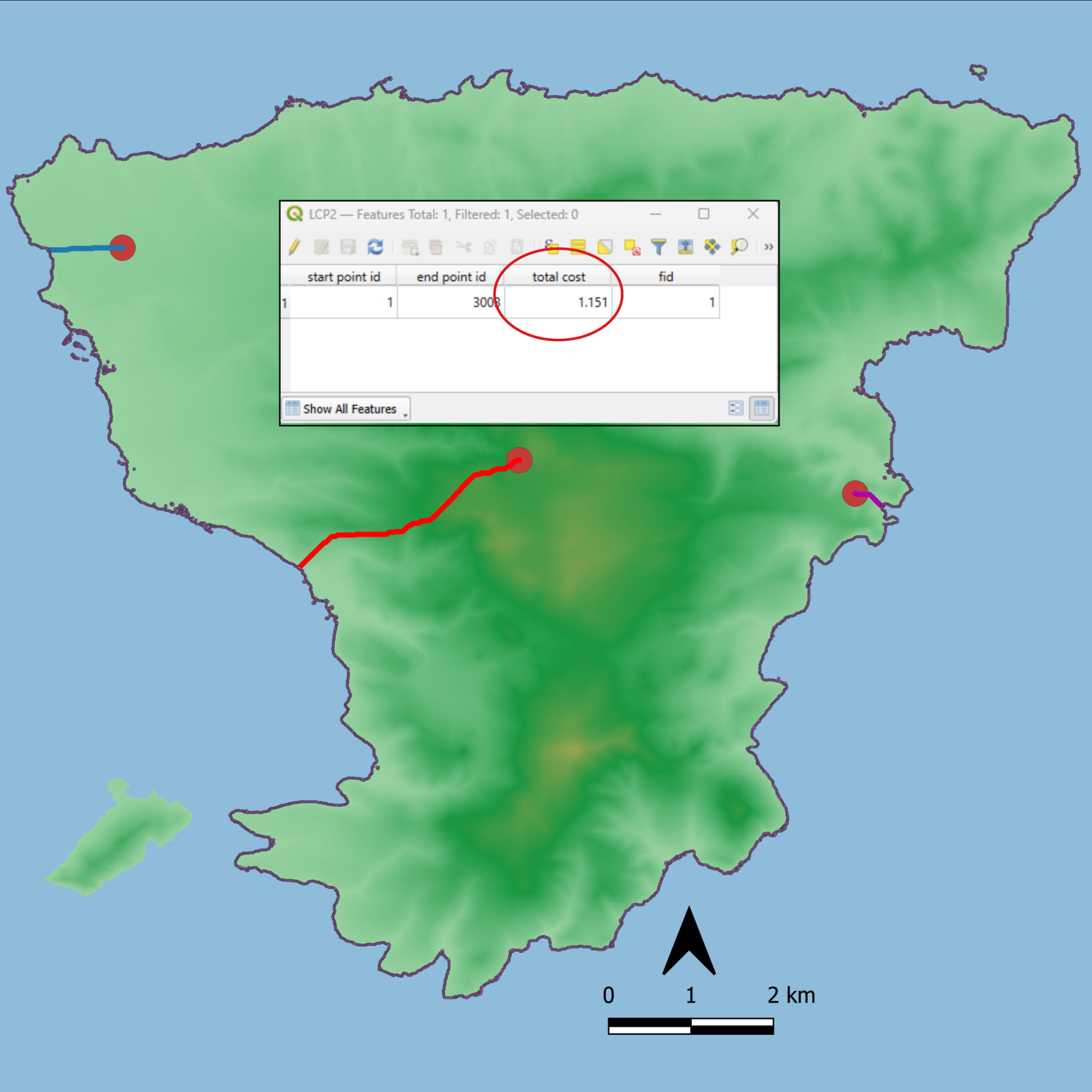
The resulting shapefile(s) can be inspected for a value listed under “Total Cost” (Right-click layer→Open Attribute Table). This is the cost of the movement based on the Cost Surface.
30s
Copy the “Total Cost” value into your database processor (i.e. Excel, Calc) of choice.
1m
Convert from hours to minutes by multiplying the value by 60. This is now the Coastal Proximity Value (CPV) in minutes. Use the CPV to quantify the temporal and spatial relationship between a site and the ancient shoreline.
5m
F. Data Interpretation
With this data, you can identify periods of greater or lesser coastal proximity in settlement patterns.
Troubleshooting and Validation
Check for zero slope cells to avoid misleading cost values.
Validate results with ethnographic or historical route data if possible.
Make sure to remove false positive inland areas that may have an elevation of “1 m”. See also “B. Shoreline Delineation.”
Output
Tabulate the median or average time-cost for sites within different chronological phases to check on larger-scale patterns in Coastal Proximity (see e.g. Nuttall 2024a; 2024b).
Protocol references
Nuttall, C. 2024a. “A GIS Analysis of Coastal Proximity with a Prehistoric Greek Case Study.” JCAA, Journal of Computer Applications in Archaeology, Vol. 7, Issue 1, pp. 170–184. https://doi.org/10.5334/jcaa.143
Nuttall, C. 2024b. “In the Shadows of a Giant?’ A Spatial Analytical Method for Assessing Coastal Proximity using R: a Case-Study from the Bronze Age Saronic Gulf (Greece).” Virtual Archaeology Review, Vol. 31, pp. 16–36. https://doi.org/10.4995/var.2024.21694
Acknowledgements
I would like to acknowledge Jovan Kovacevic for discussions concerning the method. I would also like to thank the Swedish Research Council for their generous funding on the International Postdoc in Humanities and Social Sciences (2023-2025) during which time this method was created.