May 04, 2026
Calibrating a blue light source with Dronpa-2
This protocol is a draft, published without a DOI.
- Aliénor Lahlou1,2,
- Sébastien Marino1,
- Emma Simon2,
- Théo Beguin2,3,
- Hélène Merceron2,
- Mrinal Mandal2,
- Marie-Aude Plamont2,
- Thomas Le Saux2,
- Ludovic Jullien2
- 1Paris Research, Sony Computer Science Laboratories – Paris, 75005, France;
- 2AIV, Department of Chemistry, École Normale Supérieure, PSL University, Sorbonne University, CNRS, Paris, France;
- 3Université Paris-Saclay, CNRS, Institut de Chimie Physique, UMR CNRS 8000, 91405, Orsay, France
- DREAM


External link: https://github.com/DreamRepo/light_calibration
Protocol Citation: Aliénor Lahlou, Sébastien Marino, Emma Simon, Théo Beguin, Hélène Merceron, Mrinal Mandal, Marie-Aude Plamont, Thomas Le Saux, Ludovic Jullien 2026. Calibrating a blue light source with Dronpa-2. protocols.io https://dx.doi.org/
Manuscript citation:
Lahlou, A., Tehrani, H.S., Coghill, I. et al. Fluorescence to measure light intensity. Nat Methods 20, 1930–1938 (2023). https://doi.org/10.1038/s41592-023-02063-y
License: This is an open access protocol distributed under the terms of the Creative Commons Attribution License, which permits unrestricted use, distribution, and reproduction in any medium, provided the original author and source are credited
Protocol status: Working
We use this protocol and it's working
Created: November 24, 2025
Last Modified: May 04, 2026
Protocol Integer ID: 233323
Keywords: Irradiance, Light intensity, Actinometry, Fluorescence, Imaging, Inner filter effect, Calibration of setting scales in optical instruments, Spectral measurement of light intensity, fluorescence intensity, retrieval of the light intensity, light intensity, blue light source, constant illumination, wide ranges of wavelength, wavelength, depth of sample
Funders Acknowledgements:
Morphoscope2
Grant ID: ANR-10-INBS-04
IPGG
Grant ID: ANR-11-EQPX-0029
PSL
Grant ID: ANR-10-IDEX-0001-02
EIC Pathfinder DREAM
Grant ID: 101046451
Abstract
Quantitative measurement of light intensity is required in many fields of biology, chemistry, engineering, and physics. The available protocols necessitate specific equipment and expertise, and suffer from limitations in their scope. Here we report on a protocol, which exploits fluorescence to enable the retrieval of the light intensity even in the depth of samples, with spatial distribution information, over wide ranges of wavelengths and intensities, and in a quick, inexpensive, and simple manner. It relies on species whose fluorescence intensity follows a
mono-exponential decay or rise under constant illumination.
Image Attribution
Sébastien Marino, Sony CSL Paris
Guidelines
This protocol will allow you to calibrate a blue light source using the green fluorescent actinometer Dronpa-2. It will explain how to proceed with the calibration but also produce Dronpa-2 to prepare the samples.
Materials
Light source to calibrate in the range [445 nm,500 nm].
Scale to prepare the solutions
Brown glassware or Aluminium foil to keep the solutions in the darkness
Spectral data available online https://github.com/DreamRepo/light_calibration/tree/main/spectra_plotly
Fluorimeter or any optical instrument, which can measure and record the time evolution of the fluorescence signal from the fluorescent actinometer
Quartz cuvette or glass microscope slides with a 100 µm spacer to build a chamber
Software for fitting the time evolution of the fluorescence response to illumination (example: https://github.com/DreamRepo/light_calibration)
Solvant composition: DPBS pH 7.4 buffer (2.7 mM KCl, 138 mM NaCl, 1.5 mM KH2PO4, 8.1 mM Na2HPO4) or Tris buffer pH 7.4 (50 mM Tris, 150 mM NaCl)
Dronpa-2 plasmid: TODO
Troubleshooting
Problem
No time evolution of the fluorescence signal from the final solution of fluorescent actinometer under constant illumination:
Solution
- Check that the actinometer has been kept at 4°C under the protection from ambient light.
- Check that the sampling rate is adapted to the light intensity: fluorescence may decay too quickly to be captured.
- The excitation wavelength may not correspond to the absorption range of the actinometer.
Problem
The cross section σ at an excitation wavelength belonging to the wavelength range of relevance for a given fluo- rescent actinometer is not tabulated in the reported Table
Solution
A good estimate can be retrieved from relative absorption coefficient of Dronpa-2 by exploiting the cross sections at the closest tabulated value as follows: σ(λuncal)=σ(λcal)ε(λcal)/ε(λuncal) where λuncal is the wavelength at which there is no tabulated value for σ, λcal is the closest wavelength at which σ has been calculated and ε is the absorption coefficient of Dronpa-2. The ratio ε(λcal)/ε(λuncal) can be calculated as A(λcal)/A(λuncal) with A the absorption using the absorption spectrum of Dronpa-2 available at this link:
https://github.com/DreamRepo/light_calibration/blob/main/spectra_plotly/Dronpa%202.csv
Problem
The fluorescence is increasing and not decreasing when turning on the blue light.
Solution
Dronpa-2 is reversibly photoswitchable fluorescent actinometers, and relaxes in the dark. The light intensity I obeys: I (λexc) = (1 − k∆τ)/στ, where k∆ is the rate constant associated to thermal relaxation after photoconversion (expressed in s−1). Hence, I = 1/στ for retrieving I implies that k∆τ ≪ 1, which has to be checked. k∆ is equal to 0.02 s−1 for Dronpa-2 around room temperature.
Problem
Blurred intensity map
Solution
For calibration of light intensity in fluorescence imaging, the intensity retrieval is strictly valid when the actinometer molecules do not move. However, when they can diffuse (diffusion coefficient D), the spatial resolution of the intensity is then limited to sqrt(Dτ). The faster the photoconversion, the higher the spatial resolution. At the limit of homogenization (e.g. upon stirring), the spatial information of the illumination profile is lost and one can retrieve the overall amount of light intensity I received by the actinometer solution from the measured overall relaxation time τ.
Problem
The kinetic of photoswitching isn't monoexponential
Solution
As for the problem of blurred intensity map, it’s probably a matter of homogeneity. When the kinetic is recorded, free diffusion between illuminated and unilluminated areas induce merging of measurement of Dronpa-2 molecules at different time courses of photoswitching, creating a multiexponential profile. A monoexponential profile can be retrieved by immobilising molecules, restricting its localizations in a zone where the light is homogeneous or stirring the whole solution. In the last case, the measured light intensity <I> correspond to an average value taking into account both illuminated and unilluminated areas. The intensity I truly delivered by the light source can be estimated as I=<I>Atot/Ai with Ai the illuminated area and Atot the total area of the surface of the sample facing the light.
Problem
The light intensity value measured is much lower compared to the one expected (2-4 orders of magnitude)
Solution
It is possible that the photoswiching reaction is too fast and occurs within the first point of measurement with a given recording setup. In that case, it is possible to see the very slower photobleaching kinetic of a fraction of Dronpa-2 that remained in the “ON” state, which is another reaction that can’t be simply linked to the light intensity. Then if you have an idea of the order of magnitude of the light intensity of your setup and that you see an abnormally slow kinetic with a pretty weak signal, you are probably recording the residual photobleaching instead of the characterized photoswitching reaction. To record the correct kinetics, you should try to increase the measurement rate as much as possible and/or reduce the light intensity to slow down the reaction, while ensuring that you remain within the power linearity range of the source being used. If the photoswitching is still too fast, a neutral density filter with a known attenuation factor can be inserted into the optical path of the setup to further slowdown the reaction, allowing for the measurement of a reduced light intensity from which the actual light intensity can be deduced.
Before start
You will need:
- the ability to produce Dronpa-2 which is not commercially available yet.
- a blue light source you wish to calibrate.
- the ability to record the fluorescence across time (example: video, acquisition of the signal of a photodiode)
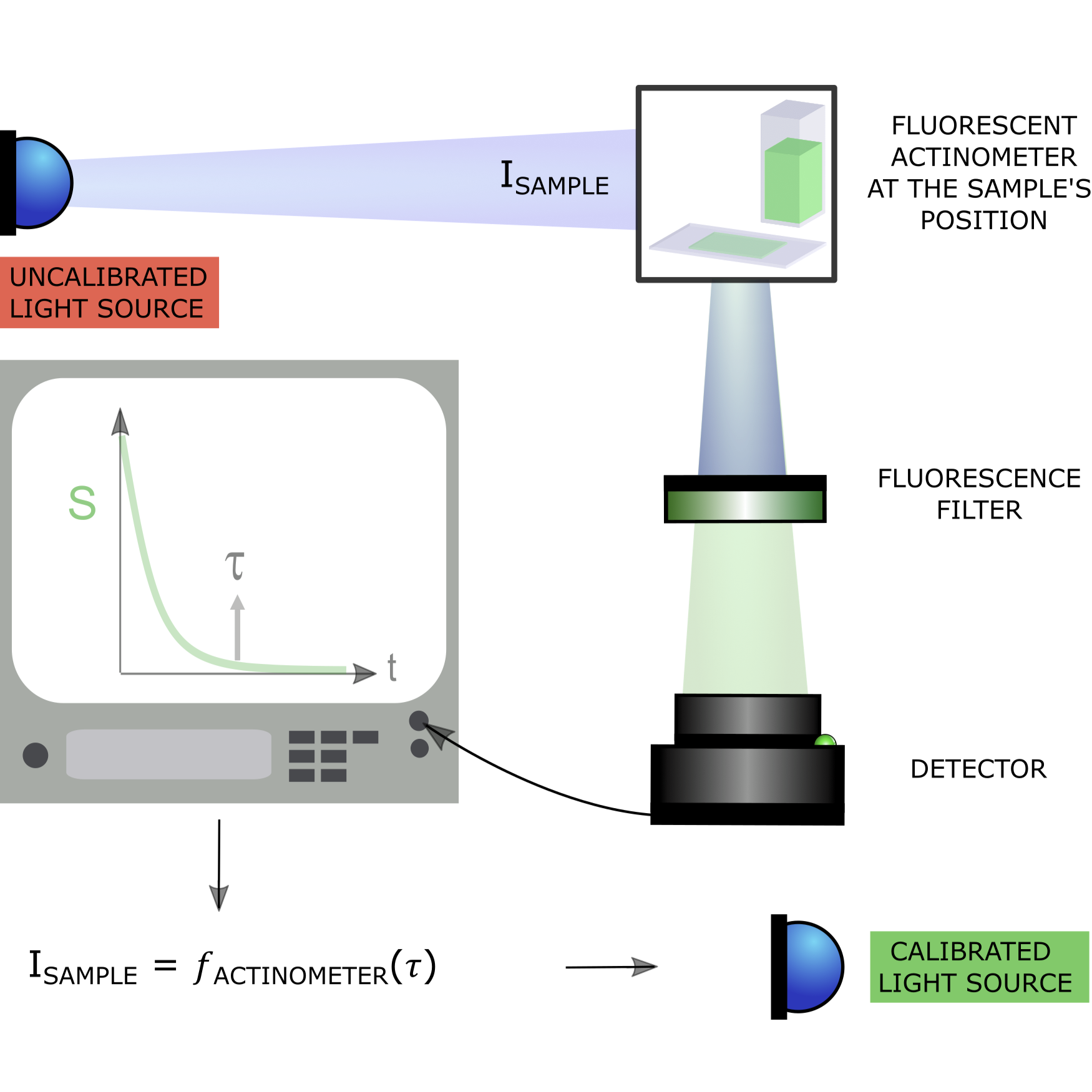
Fluorescence acquisition
3m
After preparing the sample of choice according to the section "Sample preparation" at the end of the document, perform the following steps:
Configure your fluorescence imaging set-up according to the excitation and emission spectra of Dronpa-2, presented below:
Note
Absorption and emission spectra of the Dronpa-2 protein:
An example for acquisition parameters: excitation light (the one to calibrate) at 480 nm, emission filter at 515 nm (corresponding to a GFP filter). Good quality filters are required for this calibration otherwise the input light reflected or transmitted (depending on the setup configuration) will submerge the signal of interest.
Note
General principle of the calibration:
You can use a camera or a photon counter as the detector.
An example of calibration configuration on an epifluorescence microscope.
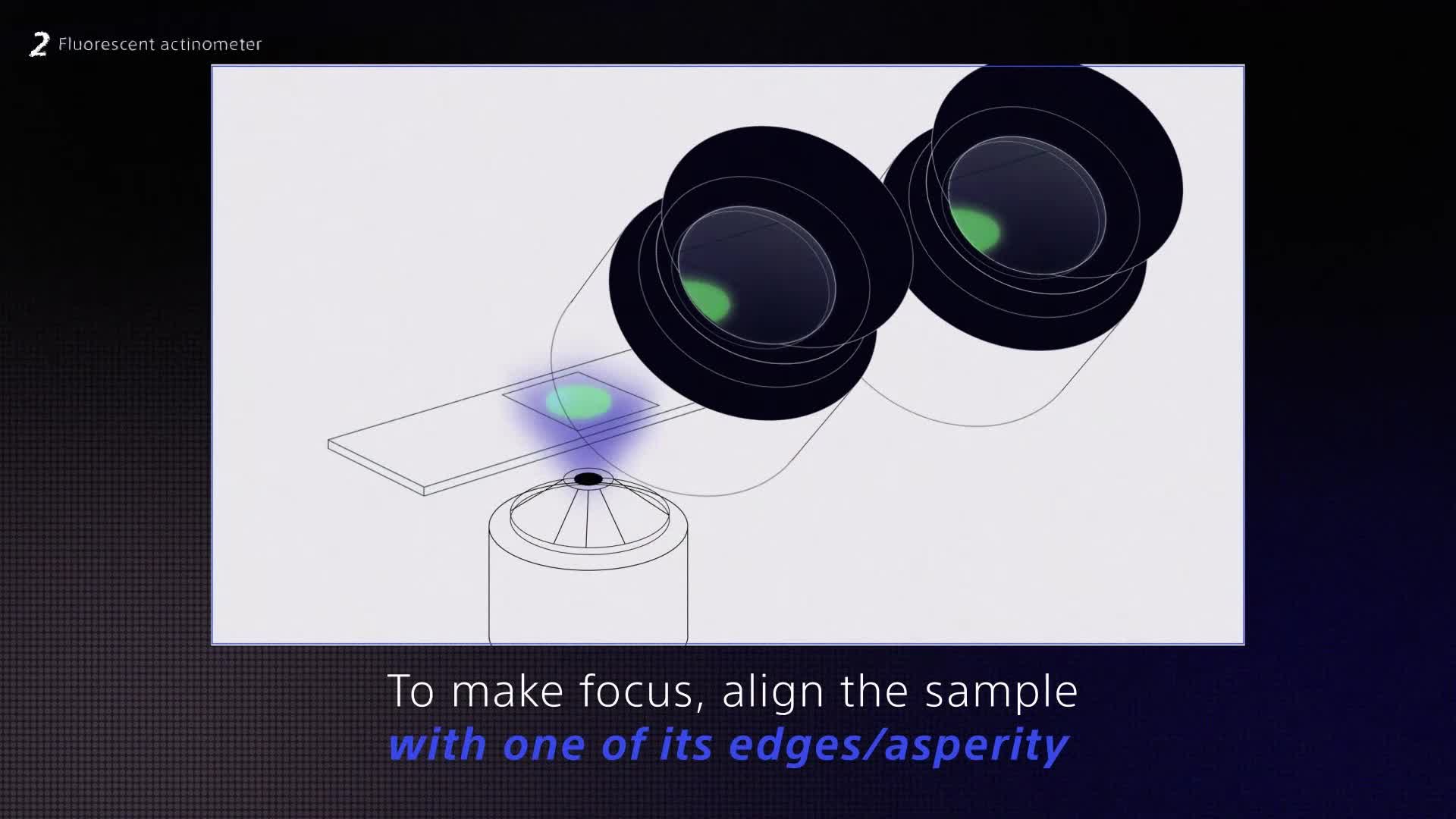
Then, place your sample on your set-up and focus at the sample.
Note
Advice to perform the focus:
Brightfield imaging is convenient for a first focus.
Alternatively, in fluorescence mode:
Since the fluorescence decays with blue light, the sample can be hard to observe. Several options are possible to simplify this step :
- Co-illuminate with a violet light (405 nm). Violet light prevent the fluorescence decay of fluorescence of Dronpa-2 under blue light.
- Add green fluorescent beads in the sample.
In all cases use edges and asperities of the sample to facilitate the focus.
Once the focus is performed, let the sample sit in the dark to recover its fluorescence (3 minutes are enough for thermal recovery of the fluorescence) and then expose the sample with a time constant monochromatic light at wavelength λexc in the [445nm - 500nm] wavelength range (i.e. in the absorption band of Dronpa-2).
As the fluorescence of Dronpa-2 decays quickly, you need to trigger the acquisition of the fluorescence at the same time the excitation light is switched on and adapt the acquisition rate.
Note
The recovery of the fluorescence can also be performed in few seconds with illumination around 400 nm to trigger the photochemical back reaction. It can be very usefull to quickly record several decays in a row.
3m
Record the fluorescence intensity at λem in the [515nm - 600nm] wavelength range (i.e. in the emission band of Dronpa-2) as a function of time.
Note
The time evolution of the sample fluorescence should look like below, as an monoexponential decay.
Here, the fluorescence decay over time is recorded on an oscilloscope.

Here is presented a simulation of how would look the sample through a fluorescence microscope. The histogram present the distribution of the fluorescence intensity in each pixel.
The relaxation time τ, leading to the fluorescence decay of Dronpa-2, is linked to the light intensity.
To retrieve it, process the time evolution of the decaying fluorescence signal F(t) with the monoexponential fitting equation given below to retrieve the relaxation time :
with F0 and Finf constants depending on your acquisition.
Note
Advice to run the fit:
First, apply the unsupervised monoexponential fitting function given above over the whole acquisition window to extract a first guess of the characteristic time τ1. Then, restrict the time window to [0, 5τ1] and extract a second value τ2 using the same monoexponential fitting function. This last τ value is used in the next step to determine the light intensity.
Note
Example of Python code you can use to fit the monoexponential fluorescence intensity decay:
import numpy as np
from scipy.optimize import curve_fit
# --- Define the monoexponential model (Eq. S1) ---
def monoexp(t, F_inf, F0, tau):
"""
Monoexponential decay model:
F(t) = F_inf + (F0 - F_inf) * exp(-t / tau)
"""
return F_inf + (F0 - F_inf) * np.exp(-t / tau)
# --- Step 1: Fit over the whole acquisition window ---
def fit_tau_whole_window(t, F):
"""
Fit the monoexponential model over the entire acquisition window.
Returns tau1 (first guess).
"""
# Initial guesses: F_inf ~ last value, F0 ~ first value, tau ~ mean time
p0 = [F[-1], F[0], (t[-1] - t[0]) / 2]
popt, _ = curve_fit(monoexp, t, F, p0=p0, maxfev=10000)
F_inf, F0, tau1 = popt
return tau1, popt
# --- Step 2: Restrict to [0, 5*tau1] and refit ---
def fit_tau_restricted_window(t, F, tau1):
"""
Restrict the time window to [0, 5*tau1] and refit.
Returns tau2 (refined estimate).
"""
mask = t <= 5 * tau1
t_restricted = t[mask]
F_restricted = F[mask]
p0 = [F_restricted[-1], F_restricted[0], tau1]
popt, _ = curve_fit(monoexp, t_restricted, F_restricted, p0=p0, maxfev=10000)
F_inf, F0, tau2 = popt
return tau2, popt
# --- Example usage ---
if __name__ == "__main__":
# Simulated data for demonstration
t = np.linspace(0, 100, 200) # time points
true_params = (10, 100, 15) # F_inf, F0, tau
F = monoexp(t, *true_params) + np.random.normal(0, 2, size=t.size) # noisy data
# Step 1: whole window fit
tau1, params1 = fit_tau_whole_window(t, F)
print(f"First guess tau1 = {tau1:.3f}")
# Step 2: restricted window fit
tau2, params2 = fit_tau_restricted_window(t, F, tau1)
print(f"Refined tau2 = {tau2:.3f}")
Extract the light intensity I as I = 1/στ by using the relevant value of the cross section of Dronpa-2 photoconversion σ(λexc) given in this table: https://pmc.ncbi.nlm.nih.gov/articles/PMC10703675/table/Tab1/
If you acquire a video, you can also perform the fit pixel-per-pixel. You can use the following code available on Github.
Software
Light calibration
NAME
Aliénor Lahlou
DEVELOPER
Note
Video explanation:
We tested the Dronpa-2-based actinometric approach with three sample formats for measuring light intensity in the 440–500 nm wavelength range: a Dronpa-2 solution, Dronpa-2-labeled Escherichia coli cells, and fixed U-2 OS eukaryotic cells labeled at the nucleus.
The production of those actinometers is reported in the following STEP CASES. The plasmids for bacterial expression of Dronpa-2 carrying an N-terminal hexahistidine tag and for mammalian expression of Dronpa-2 fused at the C-terminal of the histone H2B (H2B-Dronpa-2) were previously described.
The Dronpa-2-labeled Escherichia coli cells can be kept under the protection of ambient light (container covered with an Aluminium foil) at - 20°C for up to two weeks.
The fixed U-2 OS eucaryotic cells Dronpa-2-labeled at their nucleus remain functional for several weeks when kept at +4°C.
Purification of Dronpa-2From 10 to 14 steps
The plasmids for bacterial expression of Dronpa-2 carrying an N-terminal hexahistidine tag (previously described):
Quérard, J. et al. Resonant out-of-phase fluorescence microscopy and remote imaging overcome spectral limitations. Nat. Commun. 8, 969 (2017)
Querard, J. et al. Photoswitching kinetics and phase sensitive detection add discriminative dimensions for selective fluorescence imaging. Angew. Chem. Int. Ed. 54, 2633–2637 (2015).
Dronpa-2 is a variant of Dronpa with the mutation M159T. The gene encoding Dronpa-2 was kindly provided by Stefan Jakobs. The plasmids for bacterial expression of Dronpa-2 carrying an N-terminal hexahistidine tag was obtained by cloning their genes in the pProEX vector: the sequence coding for Dronpa-2 was inserted between Ehe I and Hind III.
The Dronpa-2 plasmid with an N-terminal hexahistidine tag was transformed in E. coli BL21 strain. Cells were grown in Terrific Broth (TB) supplemented with ampicillin (100 μg/mL) at 37°C.
The expression was induced at 30°C or 16°C by addition of isopropyl β-D-1-thio-galactopyranoside (IPTG) to a final concentration of 1 mM at OD(600)=0.6.
16h
The cells were harvested after 16 h of expression and lysed by sonication in lysis buffer (50 mM PBS with 150 mM NaCl at pH 7.4, 1 mg/ml DNAse, 5 mM MgCl2 and 1 mM phenylmethylsulfonyl fluoride (PMSF), and a cocktail of protease inhibitors (Sigma Aldrich; S8830)).
After lysis, the mixture was incubated on ice for 2 h for DNA digestion.
2h
The insoluble material was removed by centrifugation and the supernatant was incubated overnight with Ni-NTA agarose beads (Thermo Fisher) at 4°C in a rotator-mixer.
12h
The protein loaded Ni-NTA column was washed with 20 column volumes of N1 buffer (50 mM PBS, 150 mM NaCl, 20 mM imidazole, pH 7.4) and 5 column volumes of N2 buffer (50 mM PBS, 150 mM NaCl, 40 mM imidazole, pH 7.4).
The bound protein was eluted with N3 buffer (50 mM PBS, 150 mM NaCl, 0,5 M imidazole, pH 7.4).
Either:
The eluted protein was loaded onto PD-10 desalting column (GE Healthcare) for buffer exchange.
Or:
Protein fractions were dialyzed on cassette Slide-A-Lyzer Dialysis Cassettes (Thermofisher) against 50mM PBS pH 7.4, 150mM NaCl.
The final concentration depends on multiple experimental paremeters and should lie between 20mM to 400mM. It can be measured through absorbance.
Once the protein is extracted, a sample has to be prepared for observation. The sample geometry should be identical to the samples that will be observed with the device once it is calibrated.
Dilute stock Dronpa-2 solution in DPBS pH 7.4 buffer (2.7 mM KCl, 138 mM NaCl, 1.5 mM KH2PO4, 8.1 mM Na2HPO4, Thermofischer) or in Tris buffer pH 7.4 (50 mM Tris, 150 mM NaCl) to get final solutions, which exhibit an absorbance lower than 0.15 at 488 nm along the optical path ℓ in the sample configuration.
These solutions can be kept at 4°C for weeks under the protection from ambient light (e.g. by using a brown glassware enveloped in an Aluminium foil).
Microscope slide1 step
The Dronpa-2 sample is prepared the same way the sample to illuminate is prepared. Target 10-30 µM Dronpa-2 concentration.
Note
Sample preparation:
Protocol references
About actinometry:
1. H. J. Kuhn, S. E. Braslavsky, and R. Schmidt, Chemical Actinometry (IUPAC Technical Report), Pure Appl. Chem., 2004, 76, 2105–2146.
2. Lahlou, A., Tehrani, H.S., Coghill, I. et al. Fluorescence to measure light intensity. Nat Methods 20, 1930–1938 (2023). https://doi.org/10.1038/s41592-023-02063-y
Applications of actinometry protocols
1. Beguin et al. BEAM: A Custom-Built and Versatile Optical Setup for Real-Time Monitoring of Absorption and Emission Spectra During Photobleaching of Fluorescent Proteins, Chem Methods, 2026, 6, e202500097, https://doi.org/10.1002/cmtd.202500097
2. Beguin et al. Fluorescent Protein Photobleaching: From molecular processes to spectromicroscopy, Biorxiv, 2026, https://doi.org/10.64898/2026.03.31.715555
3. Eisenmann, I., L’homme, A., Lahlou, A., Bujaldon, S., Le Saux, T., Bailleul, B., ... & Jeanneret, R. (2025). Light-induced phase separation with finite wavelength selection in photophobic microalgae. Physical Review Letters, 135(14), 148401.
4. Lahlou, A., Coghill, I., Cochard, A., Ruyer-Thompson, A., Colliaux, D., Legou, T., ... & Jullien, L. (2026). Minimal reproduction and calibration of a fluorescence microscope for single-cell imaging. Journal of Open Hardware, 10(1).
5. Lahlou, A., Orlando, M., Bujaldon, S., Gaultier, W., Israelievitch, E., Hanappe, P., ... & Bailleul, B. (2026). Interplay between high‐energy quenching and state transitions in Chlamydomonas reinhardtii: a single‐cell approach. New Phytologist.
About fluorescence:
B. Valeur, M.-N. Berberan-Santos, Molecular Fluorescence: Principles and Applications 2nd Edition, Wiley, 2012.
About Dronpa-2 (plasmids):
1. J. Querard, R. Zhang, Z. Kelemen, M.-A. Plamont, X. Xie, R. Chouket, I. Roemgens, Y. Korepina, S. Albright, E. Ipendey, M. Volovitch, H. L. Sladitschek, P. Neveu, L. Gissot, A. Gautier, J.-D. Faure, V. Croquette, T. Le Saux, L. Jullien, Resonant out-of-phase fluorescence microscopy and remote imaging overcome spectral limitations, Nat. Commun., 2017, 8, 969.
2. Querard, Jérôme, et al. "Photoswitching kinetics and phase‐sensitive detection add discriminative dimensions for selective fluorescence imaging." Angewandte Chemie 127.9 (2015): 2671-2675.
Alternative RSFP for actinomtery (supplementary materials):
R. Chouket, A. Pellissier-Tanon, A. Lahlou, R. Zhang, D. Kim, M.-A. Plamont, M. Zhang, X. Zhang, P. Xu, N. Desprat, D. Bourgeois, A. Espagne, A. Lemarchand, T. Le Saux, L. Jullien, Extra kinetic dimensions for label discrimination, Nat. Commun., 2022, 13, 1482;
About data processing:
Mechanistic reduction leading to monoexponential fit of the time evolution of the fluorescence signal: R. Chouket, A. Pellissier-Tanon, A. Lahlou, R. Zhang, D. Kim, M.-A. Plamont, M. Zhang, X. Zhang, P. Xu, N. Desprat, D. Bourgeois, A. Espagne, A. Lemarchand, T. Le Saux, L. Jullien, Extra kinetic dimensions for label discrimination, Nat. Commun., 2022, 13, 1482
Acknowledgements
The authors thank Anumita Jawahar, Claude Boccara, Nathalie Gaudreault, Roland Nitschke and Quarep-LiMi Working Group 1 members for useful advice.