Aug 27, 2025

Public workspaceBioinformatic workflow for Nanopore metabarcoding analysis

Bioinformatic workflow for Nanopore metabarcoding analysis
  • Juan M Zurita-Artaloitia1,
  • Ilse Patricia Salinas Peralta2,
  • Alejandra Escobar-Zepeda3,
  • Jérôme rleyen2,
  • Alejandro Sanchez2,
  • Liliana Pardo-López1
  • 1Instituto de Biotecnología - UNAM;
  • 2UUSMB/UNAM;
  • 3EBI
Icon indicating open access to content
QR code linking to this content
Protocol CitationJuan M Zurita-Artaloitia, Ilse Patricia Salinas Peralta, Alejandra Escobar-Zepeda, Jérôme rleyen, Alejandro Sanchez, Liliana Pardo-López 2025. Bioinformatic workflow for Nanopore metabarcoding analysis. protocols.io https://dx.doi.org/10.17504/protocols.io.eq2lywmxqvx9/v1
License: This is an open access protocol distributed under the terms of the Creative Commons Attribution License,  which permits unrestricted use, distribution, and reproduction in any medium, provided the original author and source are credited
Protocol status: Working
We use this protocol and it's working
Created: October 17, 2024
Last Modified: August 27, 2025
Protocol Integer ID: 110247
Keywords: nanopore, barcoding, 16s, diversity, bioinformatic workflow for nanopore, oxford nanopore, nanopore, metabarcoding analysis, barcoding experiment, bioinformatic workflow, alpha diversity analysis between sample, alpha diversity analysis, sequencing run, rarefaction curve
Funders Acknowledgements:
CONACYT Scholarship
Grant ID: 1270074
LANCO-CONAHCyT
Grant ID: APOYOSLNC-2023-80
DGAPA-PAPIIT
Grant ID: IG200223
Disclaimer
None
Abstract
This protocol is aimed to help scientists process an Oxford Nanopore sequencing run from a 16S meta-barcoding experiment to produce a rarefaction curve, an alpha diversity analysis between samples and a stacked bar plot of the most represented taxons.
Guidelines
If its your first time using a Linux environment, you should check a basic Linux tutorial first or ask for help to a colleague.

Materials
Software used in this specific workflow:
  • A Linux/Mac terminal with Ubuntu 22.04.5
(In case you are using Windows: a Linux virtual machine will work (But you may need to manually install some dependencies that are installed by default in Linux/Mac)).
  • R v. 4.4.2
  • R Studio v. 2024.04.2
  • Perl v 5.32.1
  • Porechop v. 0.2.4
  • FastQC v. 0.11.9
  • Chopper v. 0.8.0
  • Parallel-meta 2 v. 2.4.1
  • Metaxa2 Database v.  2.2.3

The R libraries used in this analysis are:
  • RColorBrewer
  • vegan
  • tidyverse
  • tibble
  • cowplot
  • ggh4x
  • factoextra
  • reshape2
  • dplyr
  • microbiome
  • ggplot2
  • ranacapa
  • microViz
  • microbiomeutilities
Troubleshooting
Safety warnings
Running Parallel-meta in a low-specs machine may cause trouble to the hardware.
Considerations
Software used in this specific workflow:
  • A Linux/Mac terminal with Ubuntu 22.04.5
(In case you are using Windows: a Linux virtual machine will work (But you may need to manually install some dependencies that are installed by default in Linux/Mac)).
  • R v. 4.4.2
  • R Studio v. 2024.04.2
  • Perl v 5.32.1
  • Porechop v. 0.2.4
  • FastQC v. 0.11.9
  • Chopper v. 0.8.0
  • Parallel-meta 2 v. 2.4.1
  • Metaxa2 Database v.  2.2.3
  • Apptainer v. 1.4.0
  • Taxonkit v.0.18.0
The R libraries used in this analysis are:
  • RColorBrewer
  • vegan
  • tidyverse
  • tibble
  • cowplot
  • ggh4x
  • factoextra
  • reshape2
  • dplyr
  • microbiome
  • ggplot2
  • ranacapa
  • microViz
  • microbiomeutilities
Software
R programming language
NAME
The R Foundation
DEVELOPER
To install any library you need to use the following command in the R terminal:

Command
new command name
install.packages("NAME")

Go to is very computational demanding.
If you dont't run Parallel-meta2 in a high-end computer or in a cluster, consider that the processing may take a long time.
When the commands in this tutorial have a name (The ones that end with ".sh" or ".pl"), you need to download them and run the command in your terminal.
If the command doesn't have a name, then you can simply copy and paste it directly at the terminal.
A sample data set to follow along this protocol can be obtained in the following repository:
Pre-processing data
IMPORTANT: If your data isn't coming from a Nanopore sequencer, and you already have the fastqs, skip to "Primer Cleaning".
After you extract the fastQ files from the MinION device, locate the files in the drive in your machine.

Note
The MinION device gives you the option to automatically "base call" the reads, meaning it does the signals interpretation as nucleotides. In case you didn't select that option or want to manually do the base calling, then you can do it using a software like Dorado for the task.


Copy only the desired barcodes files into your local PC. For example: the barcodes 12, 24, 36 and 48.
Command
new command name
cp -r barcode12 barcode24 barcode36 barcode48 ~/PATH-to-store-barcodes
Verify that the directories aren't empty and have the right amount of files (Relative to the the sequencing run time).
Note
The Nanopore sequencing will usually generate a lot of barcodes because of sequencing errors. But this can be easily identified by entering the non-desired directories and checking the number of files and the number of lines in each file.
For example:
The line count for the files in the barcode02 goes from 1 to 9.
The line count for the barcode12 goes from 2,835 to 2,659,653
Inside each file you can check this lengths using the command:
wc -l *


Optional: Verify that the files are actual Nanopore reads.
Command
new command name
zcat FAW16131_pass_barcode12_1dba8d5b_de32243e_0.fastq.gz | head -2
The result should look like this:

@90c28ef6-45c8-4631-8851-2a67f74df137 runid=de32243e9f191a1a220f17ceaf869f23af588111 read=30 ch=324 start_time=2024-06-14T08:27:37.190699-06:00 flow_cell_id=FAW16131 protocol_group_id=Sigsbee24 sample_id=1 barcode=barcode12 barcode_alias=barcode12 parent_read_id=90c28ef6-45c8-4631-8851-2a67f74df137 [email protected]
GCCGTCCATGGCCGCCGTTCCAGTTACGTATTGCCAATTGCTGCAGGTAGAAAACAGAATCGGATTAACCTACTTGCCTGTCGCTCTATCTTCCGGTTACCTTGTTACGACTTCCACCCCAGTCATGAACCACACCGTGAAATCGTCCCTCCCGAAGGTTAGACTAACTACTTCTGGTGCAATCCCGCACTCCCATGGTGTGACGGGCGGTGTGTACAAGGCCCGGGAACGTATTCACCGCGACATTCTGATTCGCGATTTTAAGCGATTCCGACTTCGGAGTCGAGTTGCAGACTCCGATCCGGACTACGACGCGTTTTAAAGGGATTGGCTCACTCTCGCGAGTTGGCAGCCCCTCTGTACGCGCCATTGTAGCACGTGTGTAGCCCCTGGCCGTAGGGTGACCTGACGTCATCCCCACCTTCCCCTCGGTTTGTCACCGGCAGTCTCCCTGGAGTTCTCAGCATTACCTGCTAGCAACCAGGGATAGGGGTTATACGACACGAGCTGACGACGGCCATGCAGCACCTATCCCTGGTTGCTGGCAGGCTCGGCGTTGCACCTAAATGACCTGCTCTTGGCTCCGCCTCTTCCGTGGCTGGCTGTCGCGAATCATCACCCATTCCTTCAGATGGTACTGAAATGACCAGTCGGAACATTTCCCGGTGTGGTGTCATGTTCATGACCGAATTCTGCCTAACTACTACAGCTTTCAACTTC

Concatenate all the files.
Note
Make sure you are inside the correct directory and name the concatenated output accordingly.

Command
new command name
zcat * > barcode12.fastq.gz
Once you have them all concatenated with each file being named after the barcode, store them into the same directory.
Primer cleaning
Proceed to removing the Nanopore adapter sequences from our files.

Install the following software.
Software
Porechop
NAME
CentOS 7.4.1708
OS
Ryan Wick
DEVELOPER

Run this loop. Which iterates over all the fastq files and removes the adapters, generating for each an output with the "pc" name, meaning that they have been through Porechop.
Command
Run Porechop
for name in ./*.fastq.gz; do

porechop-runner.py -i "$name" -o "${name}.pc.fastq.gz"

done

Quality check
To assure the quality of the reads, a QC step is necessary.
Install the following software:
Software
FastQC
NAME
Simon Andrews
DEVELOPER

Run the following command.
Command
new command name
fastqc -o ./FastQC_results *.pc.fastq.gz
Now check your quality results and consider if the length of your results is adequate, the quality and length of the reads.
Note
If your reads are not bigger than 1,000 bp those may not be complete 16S reads.
If your reads are bigger than 2,000 bp, those may be 16S chimeras.

Sequence filtering
Filter your sequence length with Chopper.

Software
Chopper
NAME
Ubuntu 22.04
OS
Wouter De Coster
DEVELOPER

Here, we are selecting the sequences that have a have a minimum length of 1000 and a maximum length of 2000. These lengths were selected because they are within the common lengths of 16S genes.
Command
new command name
chopper --minlength 1000 --maxlength 2000 -i $FILE > $output

Note
The filters can be variable. Depending on the quality and lengths you are looking for. This is just an example of how to filter with these parameters.
If desired, a quality filter can be done with the option:
--quality 6
(In this example, we use reads with a Phred score above 6 )
We did not consider quality in this protocol because Parallel-Meta 2 has an internal filter that removes sequences that do not resemble 16S genes.

Optional: After this step run FASTQC again, Go to to ensure that chopper worked.

Running parallel-meta
Now run the taxonomical analysis with Parallel-Meta 2, and the database Metaxa2.


Install the following software:
Software
Parallel-Meta
NAME
CentOS 7.4.1708
OS
Xiaoquan Su
DEVELOPER

As this software is no longer available, an image was uploaded here:
The image can be run with Apptainer, which can be downloaded here:
Then, this is how it can run:

Command
new command name
$ apptainer exec ./pm2.sif parallel-meta -h

Download the DB Metaxa2. Assing as "X" in the database index.

Unzip your data before using parallel-meta.

Command
new command name
gunzip *

Run the following command.
Note
This process is very computational demanding. Make sure to run it in a powerful enough computer or ask assistance from the computer expert in your research center.
A cluster with a scheduling system is highly recommended.

Command
new command name
for name in ./*.fastq; do


parallel-meta -r ${name}.fastq -d X -e 1e-30 -o "${name}_parallel"

done

Computational step
The previous step generates a directory for each barcode/sample.
Data parsing
For the next step, we need to make a loop that produces a count matrix for each classification file.
Now we edit the name of each file with the sample name, making sure each has a the termination "classification.txt"
First, make sure to be in the directory that contains all the directories created in the Go to .
After, create a file named classification_list in which all the paths to the classification files are saved.
Command
new command name
find . -name '*classification.txt' | sed 's/.txt//' > classification_list

Now, we use this command to make the loop and prepare the count matrix for each classification file.
Command
count.matrix.sh
#!/bin/bash

while read name; do

cut -f5 ${name}.txt | grep -v 'Classification' |sort | uniq -c | sort -nr | sed 's/; /;/g; s/;$//' | sed 's/^ \+//' | sed 's/ /\t/' | awk -F '\t' '{print $2 "\t" $1}' > ${name}_count_matrix.txt


echo "Finished for ${name}"

done < classification_list

Now we do the same that in step 23, making now a path list file but for each matrix.

Command
new command name
find . -name '*classification_count_matrix.txt' > matrix_list.txt


Command
matrix.integrator.perl
#!/usr/bin/perl
use strict;
use warnings;

scalar@ARGV == 1 || die "usage: $0 <file_list.txt>
      file_list.txt      List of input files, each one is a matrix with the same format:
                         - No header
                         - Lineage is in the first column separated by ';'
                         - Abundance in integer numbers in the second column
";

my $files = $ARGV[0];
my @names;
my %each_matrix;
open (VALUES, $files) or die ("I can not open the file $files\n") ;
while (<VALUES>) {
	chomp;
	my $name = $_;
	PARSE($name);
	push(@names, $name);
}
close(VALUES);

## Print the matrix
open MATCOUNT, ">tmp" or die ("I can not create the file integrated_matrix.txt, check write permissions on current directory\n"); 
my $header = join("\t", @names);
print MATCOUNT "SampleID\t$header\n"; #<STDIN>;

my $lastname=scalar@names;
my $cont_names=1;
foreach my $tax (sort keys %each_matrix) {
	print MATCOUNT "$tax\t";
	foreach my $file (@names) {
		if ($each_matrix{$tax}{$file}) {
			print MATCOUNT "$each_matrix{$tax}{$file}\t";
		} else {
			print MATCOUNT "0\t";
		}
	}
	print MATCOUNT "\n";
}
close(MATCOUNT);

system("sed 's/\t\$//' tmp > integrated_matrix.txt && rm tmp");

### Subroutine to parse the file
sub PARSE {
	my $file=shift;
#	my @new_array=();
	open (FILE, $file) or die ("I can not open the file $file\n") ;
	while (<FILE>) {
		chomp;
		my($taxo, $abundance)=split('\t', $_);
#		my@lineage=split(/;/, $taxo);
#		foreach my$each_name (@lineage){
#			if ($each_name !~ /epsilon_subdivisions/ and $each_name !~ /[Gg]roup/  and $each_name !~ /unclassified/ and $each_name !~ /[Ii]ncertae_[Ss]edis/ ) {
#				push(@new_array, $each_name);
#			}
#		}
#		if (scalar@new_array == 6) {
#			my$sp=join("_", $new_array[-1], "sp\.");
#			push(@new_array, $sp);
#			$taxo=join(";", @new_array);
#		}else{
#			$taxo=join(";", @new_array);
#		}
		$each_matrix{$taxo}{$file}=$abundance;
#		@new_array=();
	}
	close(FILE);
}

Run with the following
Command
new command name
perl matrix.pl matrix_list.txt

Next, we filter the whole table to delete the hits for eukarya, mitochondria, chloroplast and other lines that we dont need.

Note
As we are only focused in 16S diversity, we are removing the chloroplast, mitochondria and eukarya sequences.


Command
new command name
sed 's/classification_count_matrix.txt//g ; s/[./]//g ;'s/\'//g' ; s/_S[0-9][0-9][0-9]//g ; s/_S[0-9][0-9]//g ; s/_S[0-9]//g ; /Eukaryota/d;/Mitochondria/d;/Chloroplast/d' integrated_matrix.txt > integrated_matrix_good.txt


Command
taxa_levels.pl
#!/usr/bin/perl
use strict;
use warnings;

scalar@ARGV == 2 || die "usage: $0 <matrix.txt> <counts|abun>

      Programa que separa una matrix de abundancias o conteos en niveles taxonomicos

      matrix.txt      Matriz de abundancias donde la primer columna es la asignacion
                      taxonomica y el resto son las abundancias para cada muestra

      counts|abun     Especificar si la matriz es de conteos crudos o abundancias, en 
                      el segundo caso, reporta la proporcion de abundancia asignada a 
                      niveles taxonomicos mas altos del corte dado

";

my $file=$ARGV[0];
my $tipo_mat=$ARGV[1];

unless ($tipo_mat =~ "counts"  or $tipo_mat =~ "abun") {
        die "El tipo de matriz solo puede ser counts o abun en minusculas\n";
}

## Armando el hash de la matriz de abundancia original
my %matrix=();
open (FILE, $file) or die ("No puedo abrir el archivo $file\n");
my $header=<FILE>;
while (<FILE>) {
	chomp;
	my@line=split('\t', $_);
	my$tax_name=shift@line;
	if (exists $matrix{$tax_name}){	
		my@sums=();
		for (my $i=0; $i<scalar@line; $i++){
			my$add=$matrix{$tax_name}[$i]+$line[$i];
			push(@sums, $add);
		}
		$matrix{$tax_name}=[@sums];
	}else{
		$matrix{$tax_name}=[@line];
	}
}
close(FILE);

my @samples=split("\t", $header);
my $samples_number=scalar@samples -1 ;

## Armando las matrices para cada nivel taxonomico
my %domain=SEPARA(\%matrix, 1, $samples_number, $tipo_mat);
open DOM, ">dom_tmp.txt";
print DOM "$header";
foreach my $dom (keys %domain){
	print DOM "$dom\t" ;
	foreach my $count (@{ $domain{$dom} }) {
		print DOM "$count\t";
	} 
		print DOM "\n";
}
close(DOM);
system("sed 's/\t\$//' dom_tmp.txt > domain_matrix.txt");
system("rm dom_tmp.txt");

my %phylum=SEPARA(\%matrix, 2, $samples_number, $tipo_mat);
open PHY, ">phy_tmp.txt";
print PHY "$header";
foreach my $phy (keys %phylum){
	print PHY "$phy\t" ;
	foreach my $count (@{ $phylum{$phy} }) {
		print PHY "$count\t";
	} 
		print PHY "\n";
}
close(PHY);
system("sed 's/\t\$//' phy_tmp.txt > phylum_matrix.txt");
system("rm phy_tmp.txt");

my %class=SEPARA(\%matrix, 3, $samples_number, $tipo_mat);
open CLASS, ">class_tmp.txt";
print CLASS "$header";
foreach my $cla (sort keys %class){
	print CLASS "$cla\t" ;
	foreach my $count (@{ $class{$cla} }) {
		print CLASS "$count\t";
	} 
		print CLASS "\n";
}
close(CLASS);
system("sed 's/\t\$//' class_tmp.txt > class_matrix.txt");
system("rm class_tmp.txt");

my %order=SEPARA(\%matrix, 4, $samples_number, $tipo_mat);
open ORD, ">order_tmp.txt";
print ORD "$header";
foreach my $ord (sort keys %order){
	print ORD "$ord\t" ;
	foreach my $count (@{ $order{$ord} }) {
		print ORD "$count\t";
	} 
		print ORD "\n";
}
close(ORD);
system("sed 's/\t\$//' order_tmp.txt > order_matrix.txt");
system("rm order_tmp.txt");

my %family=SEPARA(\%matrix, 5, $samples_number, $tipo_mat);
open FAM, ">family_tmp.txt";
print FAM "$header";
foreach my $fam (sort keys %family){
	print FAM "$fam\t" ;
	foreach my $count (@{ $family{$fam} }) {
		print FAM "$count\t";
	} 
		print FAM "\n";
}
close(FAM);
system("sed 's/\t\$//' family_tmp.txt > family_matrix.txt");
system("rm family_tmp.txt");

my %genus=SEPARA(\%matrix, 6, $samples_number, $tipo_mat);
open GEN, ">genus_tmp.txt";
print GEN "$header";
foreach my $gen (sort keys %genus){
	print GEN "$gen\t" ;
	foreach my $count (@{ $genus{$gen} }) {
		print GEN "$count\t";
	} 
		print GEN "\n";
}
close(GEN);
system("sed 's/\t\$//' genus_tmp.txt > genus_matrix.txt");
system("rm genus_tmp.txt");

my %species=SEPARA(\%matrix, 7, $samples_number, $tipo_mat);
open SPC, ">species_tmp.txt";
print SPC "$header";
foreach my $spc (sort keys %species){
	print SPC "$spc\t" ;
	foreach my $count (@{ $species{$spc} }) {
		print SPC "$count\t";
	} 
		print SPC "\n";
}
close(SPC);
system("sed 's/\t\$//' species_tmp.txt > species_matrix.txt");
system("rm species_tmp.txt");

my %subspecies=SEPARA(\%matrix, 8, $samples_number, $tipo_mat);
open SSPC, ">subspecies_tmp.txt";
print SSPC "$header";
foreach my $subspc (sort keys %subspecies){
	print SSPC "$subspc\t" ;
	foreach my $count (@{ $subspecies{$subspc} }) {
		print SSPC "$count\t";
	} 
		print SSPC "\n";
}
close(SPC);
system("sed 's/\t\$//' subspecies_tmp.txt > subspecies_matrix.txt");
system("rm subspecies_tmp.txt");

sub SEPARA {
	my %matriz_sub=%{$_[0]};
	my $level=$_[1];
	my $muestras=$_[2];
	my $type_matrix=$_[3];
	my %regresa=();
	my(@sumas, @taxa_levels, @diferencia);
	my($level_key, $pos, $diff,$taxa2print);
	my$suma_val=0;

	foreach my $llaves (sort keys %matriz_sub) {
		@taxa_levels=split(';', $llaves);

		my $tamano=scalar@taxa_levels;
		if ($tamano >= $level) {
			$pos=$level-1;
			
			if ($taxa_levels[$pos] =~ /no_rank/){
				$pos=$level;
			}
			
			$taxa2print=join(';', @taxa_levels[0..$pos]);	### variable nueva para imprimir

			if (!exists($regresa{$taxa2print})) {
				$regresa{$taxa2print}=$matriz_sub{$llaves};
			}else{ 
			
				for (my $i=0; $i<$muestras; $i++) { 
					$suma_val=$regresa{$taxa2print}[$i]+$matriz_sub{$llaves}[$i];
	            			push(@sumas, $suma_val);
				}
			$regresa{$taxa2print}=[@sumas];
			@sumas=();
			}
		}
	}

	if ($type_matrix =~ 'abun'){
		my @suma_per_sample=();
		my $suma_val=0;

		for (my $i=0; $i<$muestras; $i++) { 
			foreach my $key (sort keys %regresa){
				$suma_val=$regresa{$key}[$i]+$suma_val;
			}
			push(@suma_per_sample, $suma_val);
			$suma_val=0;
		}
	
		foreach my $cada_suma (@suma_per_sample){
			my $resta=100-$cada_suma;
			if ($resta > 0) {
				my $higher_level= sprintf "%.6f", $resta;
				push(@diferencia, $higher_level);
			}else{
				push(@diferencia, "0");
			}
		}
		$regresa{"Classified_at_a_higher_level"}=[@diferencia];
		return %regresa;
	}else{
		return %regresa;	
	}
}
And its run adding "counts" at the end.

Command
new command name
perl taxa_levels.pl integrated_matrix_good.txt counts

We format the data for phyloseq.
Command
new command name
#!/bin/bash

awk '{print $1}' species_matrix.txt > 7taxonomy_table.txt

cut -f1 species_matrix.txt > 7taxonomy_table.txt
sed 's/;/\t/g' 7taxonomy_table.txt | sed 's/SampleID/Domain\tPhylum\tClass\tOrder\tFamily\tGenus\tSpecie/g' > 7_taxonomy_table1.txt
awk 'BEGIN{ FS = OFS = "\t" } { print (NR==1? "TAXA" : "TAXA"NR-1), $0 }' 7_taxonomy_table1.txt > taxonomy_table.txt
cut -f2- species_matrix.txt > 7_otu_table.txt
awk 'BEGIN{ FS = OFS = "\t" } { print (NR==1? "TAXA" : "TAXA"NR-1), $0 }' 7_otu_table.txt > otu_table.txt

As metaxa2 database has some outdated taxas, we will use the software Taxonkit in order to update them.
Software
Taxonkit
NAME

Command
new command name
taxonkit name2taxid --data-dir $PATH/taxonkit/database/ -i 8 --show-rank taxonomy_table.txt > out_species.txt

After this step, its necessary to check for the taxons that weren't detected by taxonkit.

Command
new command name
awk -F'\t' '$9 == ""' out_species.txt

Manually look up for the species name in the Taxonomy browser from NCBI (https://www.ncbi.nlm.nih.gov/Taxonomy/Browser/wwwtax.cgi) and change the species name in the 8th column to the current one in the taxonomy_table.txt.


In the example above, the species Pseudomonas alcaligenes needs to be changed to: Aquipseudomonas alcaligenes
After all the species names are corrected, run again Go to and Go to to make sure that all the taxons were successfully corrected by Taxonkit.
Then, run again this command:
Command
new command name
taxonkit reformat --data-dir /home/pardolab/Apps/taxonkit/database/ -I 9 -f "{K}|{p}|{c}|{o}|{f}|{g}|{s}" -F out_species.txt > species_corrected.txt


Then, transform the previous output into the taxonomy table file.

Command
new command name
cut -f1,11 species_corrected.txt  | sed 's/|/\t/g' | sed "s/'//g" | sed 's/TAXA\t/TAXA    Domain  Phylum  Class   Order   Family  Genus   Specie/' > taxonomytable.txt

Now we create a file named metadata.txt with the following structure example (each column must be separated by a tab):
SampleID Origin
ID1 Water
ID2 Sediment
ID3 Soil
ID4 Saliva

A metadata file can be created with the following command (note: you can add as many meta information as necessary, as shown in the example above):
Command
new command name
head -1 integrated_matrix_good.txt | tr "\t" "\n" > metadata.txt


...
Diversity analysis
As a result, we should have 3 files:
otu_table.txt
taxonomytable.txt
metadata.txt

Software
Phyloseq
NAME

Now paste this command in the R Studio file.
Be sure to add the working directory you are in before running it in this part: setwd("/PATH").

The code should be copied into an Rstudio session, so each line is ran individually. This is because some lines need to be modified.

For each abundance, search for the following 4 lines:


Command
new command name
Class_1up = filter_taxa(Class_perc, function(x) sum(x) > 0.1, TRUE)
Class_1up
#40
Class_top = aggregate_top_taxa2(Class_perc,top = 40, level = "Class")
For each, run the first line to define the cutoff of your relative abundance.
The second line will tell how many taxas are considered after your cut off. Try to use a number between 40-60 to avoid having too many or to little taxas.
You can register this number in the third line.
And in the fourth line register this number in a variable to be used in the plot.

Also, in the line:

Command
new command name
  facet_nested(. ~ Origin + Depth + Platform , scales = "free_x",space="free_x") +
Replace "Origin", "Depth" and "Platform" with your metadata.
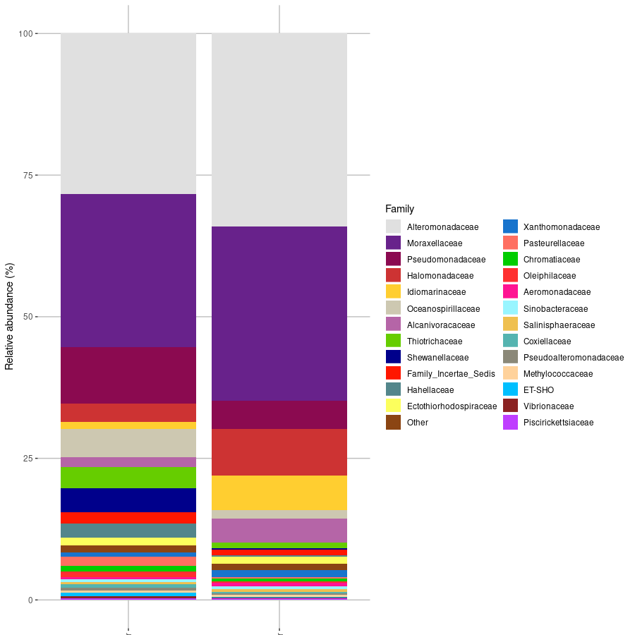
Command
new command name
#libraries
library(phyloseq)
library(dplyr)
library(vegan)
library(tidyverse)
library(tibble)
library(cowplot)
library(ggh4x)
library(factoextra)
library(reshape2)
library(dplyr)
library(microbiome  )
library(ggplot2)
library(ranacapa)
library(microViz)
library(microbiomeutilities)

#2 change working directory
setwd("$PATH_to_files")

################################################################################
#3 importar data 

#16S
otu16s_df<-read.table("otu_table.txt",
                      header=TRUE, row.names=1, check.names=FALSE)
otu16s_mat<-as.matrix(otu16s_df)
tax16s_df<-read.table("taxonomytable.txt",
                      header=TRUE, row.names=1, check.names=FALSE, sep = '\t')
tax16s_mat<-as.matrix(tax16s_df)
metadata16s_df<-read.table("metadata.txt",
                           sep="\t", header=TRUE,  row.names=1)
OTU16s = otu_table(otu16s_mat, taxa_are_rows = TRUE)
TAX16s = tax_table(tax16s_mat)
ps_16s = phyloseq(OTU16s,TAX16s, sample_data(metadata16s_df))
ps_16s

ps_16s_genus = ps_16s %>% aggregate_taxa(level = "Genus")


##### Curves ###############
fuente_rare = theme(text = element_text(size= 12, face="bold"),
                    axis.text.x = element_text(size = 12,face="bold"),
                    axis.text.y = element_text(size = 12,face="bold"),
                    panel.background = element_rect(fill = "white",colour = "grey50"), 
                    panel.grid.major = element_blank(),panel.grid.minor = element_blank())

#genus
ggrare(ps_16s_genus, step = 209, plot = T,
       parallel = T, se = F, color = "Sample" ) + 
  fuente_rare + labs(y="Géneros observados", x="Tamaño de la muestra") 


##################alpha#######################3
alphadiv <- plot_richness(ps_16s, x = "Sample",
                          measures=c("Observed","Chao1", "Shannon", "Simpson"), color = "Sample") + 
  labs(x="Origin", y="Alpha diversity")
alphadiv

##############
#16s 
genus_comp = ps_16s_genus %>% transform(transform = "compositional")
genus_perc = transform_sample_counts(genus_comp, function(x) x*100)
genus_perc
genus_1up = filter_taxa(genus_perc, function(x) sum(x) > 1, TRUE)
genus_1up
#70
genus_5up = filter_taxa(genus_perc, function(x) sum(x) > 2, TRUE)
genus_5up
#30

genus_top = aggregate_top_taxa2(genus_perc,top = 32, level = "Genus")
genus_top
data = psmelt(genus_top) # create dataframe from phyloseq object
data$Genus <- as.character(data$Genus) #convert to character
data$Genus[data$Genus == "Other"] <- "< 2% overall rel. ab."

mycolors= c( "#F6F6F6","#68228B","#2BDEBB","#C0C0C0","#EEAD0E","#CD3333",
             "#CDC8B1","#B565A7","#fff5b5","#66CD00","#53868B",
             "#fcff5d","#8B4513","#009B77","#FF6F61","#CAFF70",
             "#98F5FF","#EFC050","#FFD29B","#00BFFF","#722F37","#BF3EFF",
             "#FF1493","#096e24","#BDFFBC","#93FF33","#FF8C00",
             "#5F9EA0","#955251","#00008B","#FFD700","#CCCCFF",
             "#8B8278","#A6CF4A","#CD661D","#FF0000","#1E90FF","#CDAA7D","#D65076",
             "#FF4040","#DFFF00","#1874CD","#CD950C","#00CDCD",
             "#458B00","#FF3030","#8B6508","#cb7cc3","#76EE00",
             "#2f2aa0","#cb7c80","#92A8D1","#8B0A50","#F7CAC9",
             "#C1FFC1","#fe9000","#2BDE8A","#FA8072","#909aa6", "black")
bars_genus_top <- ggplot(data, aes(x=Sample, y=Abundance, fill=Genus)) + 
  geom_bar(aes(), stat="identity", position="stack", color="black") +
  facet_nested(. ~ Origin + Platform, scales = "free_x",space="free_x") +
  labs(x = "", y = "Abundancia relativa (%)") +
  scale_fill_manual(values=mycolors) + guides(x = guide_axis(angle = 90)) + 
  theme(panel.spacing=unit(0.1,"lines"),
        strip.background=element_rect(color="grey30", fill="grey90"),
        panel.border=element_rect(color="grey90", fill = NA),
        axis.ticks.x=element_blank()) +
  scale_y_continuous(expand = c(0.01, 0.01))
bars_genus_top

###############PHYLA####################
ps_16s_Phylum = ps_16s %>% aggregate_taxa(level = "Phylum")

Phylum_comp = ps_16s_Phylum %>% transform(transform = "compositional")
Phylum_perc = transform_sample_counts(Phylum_comp, function(x) x*100)
Phylum_perc
Phylum_1up = filter_taxa(Phylum_perc, function(x) sum(x) > 1, TRUE)
Phylum_1up
#30 y 10
Phylum_top = aggregate_top_taxa2(Phylum_perc,top = 30, level = "Phylum")
Phylum_top
data = psmelt(Phylum_top) # create dataframe from phyloseq object
data$Phylum <- as.character(data$Phylum) #convert to character
data$Phylum[data$Phylum == "Other"] <- "< 2% overall rel. ab."
bars_Phylum_top <- ggplot(data, aes(x=Sample, y=Abundance, fill=Phylum)) + 
  geom_bar(aes(), stat="identity", position="stack", color="black") +
  facet_nested(. ~ Origin + Platform, scales = "free_x",space="free_x") +
  labs(x = "", y = "Abundancia relativa (%)") +
  scale_fill_manual(values=mycolors) + guides(x = guide_axis(angle = 90)) + 
  theme(panel.spacing=unit(0.1,"lines"),
        strip.background=element_rect(color="grey30", fill="grey90"),
        panel.border=element_rect(color="grey90", fill = NA),
        axis.ticks.x=element_blank()) +
  scale_y_continuous(expand = c(0.01, 0.01))
bars_Phylum_top

############################################################################

###############Class####################
ps_16s_Class = ps_16s %>% aggregate_taxa(level = "Class")

Class_comp = ps_16s_Class %>% transform(transform = "compositional")
Class_perc = transform_sample_counts(Class_comp, function(x) x*100)
Class_perc
Class_1up = filter_taxa(Class_perc, function(x) sum(x) > 0.1, TRUE)
Class_1up
#64 y 40
Class_top = aggregate_top_taxa2(Class_perc,top = 40, level = "Class")
Class_top
data = psmelt(Class_top) # create dataframe from phyloseq object
data$Class <- as.character(data$Class) #convert to character
data$Class[data$Class == "Other"] <- "< 0.5% overall rel. ab."
bars_Class_top <- ggplot(data, aes(x=Sample, y=Abundance, fill=Class)) + 
  geom_bar(aes(), stat="identity", position="stack", color="black") +
  facet_nested(. ~ Origin + Platform, scales = "free_x",space="free_x") +
  labs(x = "", y = "Abundancia relativa (%)") +
  scale_fill_manual(values=mycolors) + guides(x = guide_axis(angle = 90)) + 
  theme(panel.spacing=unit(0.1,"lines"),
        strip.background=element_rect(color="grey30", fill="grey90"),
        panel.border=element_rect(color="grey90", fill = NA),
        axis.ticks.x=element_blank()) +
  scale_y_continuous(expand = c(0.01, 0.01))
bars_Class_top

############################################################################

###############Order####################
ps_16s_Order = ps_16s %>% aggregate_taxa(level = "Order")

Order_comp = ps_16s_Order %>% transform(transform = "compositional")
Order_perc = transform_sample_counts(Order_comp, function(x) x*100)
Order_perc
Order_1up = filter_taxa(Order_perc, function(x) sum(x) > 1, TRUE)
Order_1up
#42
Order_top = aggregate_top_taxa2(Order_perc,top = 42, level = "Order")
Order_top
data = psmelt(Order_top) # create dataframe from phyloseq object
data$Order <- as.character(data$Order) #convert to character
data$Order[data$Order == "Other"] <- "< 1% overall rel. ab."
bars_Order_top <- ggplot(data, aes(x=Sample, y=Abundance, fill=Order)) + 
  geom_bar(aes(), stat="identity", position="stack", color="black") +
  facet_nested(. ~ Origin + Platform, scales = "free_x",space="free_x") +
  labs(x = "", y = "Abundancia relativa (%)") +
  scale_fill_manual(values=mycolors) + guides(x = guide_axis(angle = 90)) + 
  theme(panel.spacing=unit(0.1,"lines"),
        strip.background=element_rect(color="grey30", fill="grey90"),
        panel.border=element_rect(color="grey90", fill = NA),
        axis.ticks.x=element_blank()) +
  scale_y_continuous(expand = c(0.01, 0.01))
bars_Order_top

############################################################################

###############Family####################
ps_16s_Family = ps_16s %>% aggregate_taxa(level = "Family")

Family_comp = ps_16s_Family %>% transform(transform = "compositional")
Family_perc = transform_sample_counts(Family_comp, function(x) x*100)
Family_perc
Family_1up = filter_taxa(Family_perc, function(x) sum(x) > 2, TRUE)
Family_1up
#30 y 10
Family_top = aggregate_top_taxa2(Family_perc,top = 35, level = "Family")
Family_top
data = psmelt(Family_top) # create dataframe from phyloseq object
data$Family <- as.character(data$Family) #convert to character
data$Family[data$Family == "Other"] <- "< 2% overall rel. ab."
bars_Family_top <- ggplot(data, aes(x=Sample, y=Abundance, fill=Family)) + 
  geom_bar(aes(), stat="identity", position="stack", color="black") +
  facet_nested(. ~ Origin + Platform, scales = "free_x",space="free_x") +
  labs(x = "", y = "Abundancia relativa (%)") +
  scale_fill_manual(values=mycolors) + guides(x = guide_axis(angle = 90)) + 
  theme(panel.spacing=unit(0.1,"lines"),
        strip.background=element_rect(color="grey30", fill="grey90"),
        panel.border=element_rect(color="grey90", fill = NA),
        axis.ticks.x=element_blank()) +
  scale_y_continuous(expand = c(0.01, 0.01))
bars_Family_top

############################################################################

###############Specie####################
ps_16s_Specie = ps_16s %>% aggregate_taxa(level = "Specie")

Specie_comp = ps_16s_Specie %>% transform(transform = "compositional")
Specie_perc = transform_sample_counts(Specie_comp, function(x) x*100)
Specie_perc
Specie_1up = filter_taxa(Specie_perc, function(x) sum(x) > 1, TRUE)
Specie_1up
#30 y 10
Specie_top = aggregate_top_taxa2(Specie_perc,top = 54, level = "Specie")
Specie_top
data = psmelt(Specie_top) # create dataframe from phyloseq object
data$Specie <- as.character(data$Specie) #convert to character
data$Specie[data$Specie == "Other"] <- "< 1% overall rel. ab."
bars_Specie_top <- ggplot(data, aes(x=Sample, y=Abundance, fill=Specie)) + 
  geom_bar(aes(), stat="identity", position="stack", color="black") +
  facet_nested(. ~ Origin + Platform, scales = "free_x",space="free_x") +
  labs(x = "", y = "Abundancia relativa (%)") +
  scale_fill_manual(values=mycolors) + guides(x = guide_axis(angle = 90)) + 
  theme(panel.spacing=unit(0.1,"lines"),
        strip.background=element_rect(color="grey30", fill="grey90"),
        panel.border=element_rect(color="grey90", fill = NA),
        axis.ticks.x=element_blank()) +
  scale_y_continuous(expand = c(0.01, 0.01))
bars_Specie_top

#genus###################
ps_16s_genus
genus_df <- data.frame(phyloseq::otu_table(ps_16s_genus))
#write.table(genus_transpose,file="genus_nmds.txt", sep = "\t", row.names = TRUE, col.names = NA)
genus_transpose_m <- as.data.frame(t(as.matrix(genus_df)))
#write.table(genus_transpose,file="genus_nmds_transpose.txt", sep = "\t", row.names = TRUE, col.names = NA)

genus_nmds <- metaMDS(genus_transpose_m, k=2, trymax=100, sfgrmin = 1e-9)
genus_nmds

stressplot(genus_nmds) # Produces a Shepards diagram
plot(genus_nmds)
genus_nmds
ordiplot(genus_nmds,type="n")
orditorp(genus_nmds,display="sites",cex=1.25,air=0.01)

This is the results for the family levels taxa, but stacked bar plots can be made in different taxa levels.
Expected result