Mar 18, 2026
Version 2
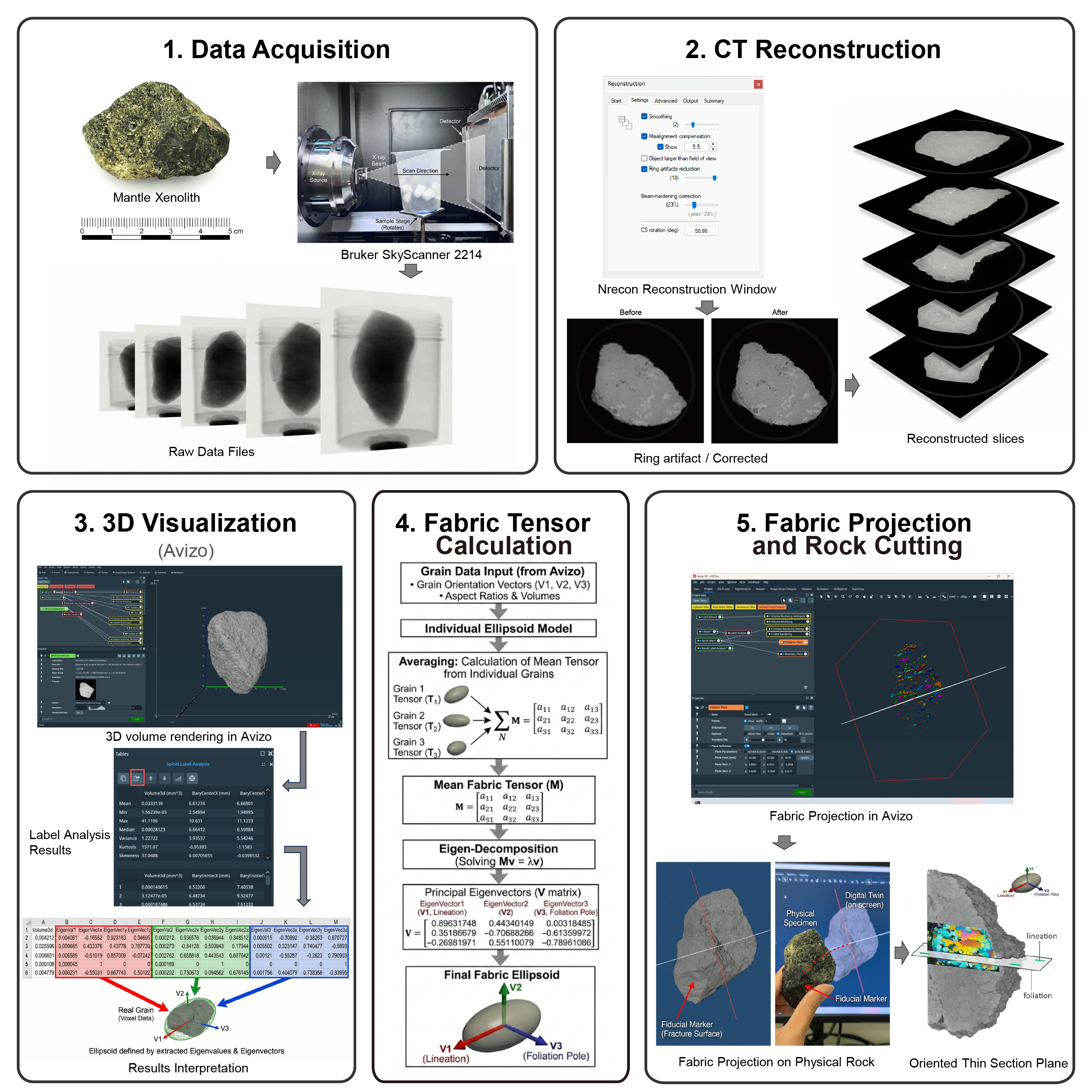
A standardized workflow for quantitative 3D shape preferred orientation analysis of minerals using X-ray computed tomography V.2
- Puqing Li1,
- Vasileios Chatzaras1,
- Matthew Foley2,
- Sinan Özaydin1,
- Patrice Rey1
- 1School of Geosciences, The University of Sydney, Sydney, NSW, Australia;
- 2Sydney Microscopy & Microanalysis, The University of Sydney, Sydney, NSW, Australia


Protocol Citation: Puqing Li, Vasileios Chatzaras, Matthew Foley, Sinan Özaydin, Patrice Rey 2026. A standardized workflow for quantitative 3D shape preferred orientation analysis of minerals using X-ray computed tomography. protocols.io https://dx.doi.org/10.17504/protocols.io.n92ld16znl5b/v2Version created by Puqing Li
License: This is an open access protocol distributed under the terms of the Creative Commons Attribution License, which permits unrestricted use, distribution, and reproduction in any medium, provided the original author and source are credited
Protocol status: Working
We use this protocol and it's working
Created: March 18, 2026
Last Modified: March 18, 2026
Protocol Integer ID: 313508
Keywords: X-ray computed tomography, Shape preferred orientation, Rock fabric, Geometric aliasing artifacts, Machine learning threshold selection, orientation analysis of mineral, standardized workflow for quantitative 3d shape, quantitative 3d shape, artificial clustering of grain orientation, reconstructing volume, sections for subsequent microstructural analysis, grain orientation, broader evaluation across other mineral phase, end workflow for quantitative 3d spo analysis, subsequent microstructural analysis, object artifacts across diverse lithology, quantitative 3d spo analysis, anisotropic physical properties of rock, computed tomography, extracting grain parameter, mineral phase, interpreting deformation process, objective minimum grain, magma flow, grain parameter, artifact mitigation, distinguishing true grain, other mineral phase, artifact, deformation process, rock type, characterization of mineral fabric, few voxel, volume threshold, mineral, object artifact, 3d, mineral fabric, preferred orientation analysis,
Funders Acknowledgements:
Australian Research Council
Grant ID: DP220100709 and LP190100146
China Scholarship Council
Grant ID: 202204910043
European Union Seventh Framework Programme
Grant ID: PIOF-GA-2012–329183
Abstract
Quantifying three‑dimensional (3D) mineral shape‑preferred orientation (SPO) is essential for interpreting deformation processes, magma flow, sediment transport, and anisotropic physical properties of rocks. X‑ray computed tomography (XRCT) enables non‑destructive, high‑resolution characterization of mineral fabrics; however, the absence of fully documented, reproducible workflows has limited broader adoption of XRCT‑based SPO analysis. A major challenge is the prevalence of small segmented objects—typically composed of only a few voxels—that generate poorly constrained ellipsoid fits and introduce geometric aliasing, producing artificial clustering of grain orientations that masks the true rock fabric.
This Lab Protocol presents a complete, end-to-end workflow for quantitative 3D SPO analysis using XRCT, focusing on automated data cleaning and artifact mitigation. The protocol guides users through optimizing acquisition settings, reconstructing volumes, and extracting grain parameters. To address geometric aliasing, we introduce a semi-supervised machine-learning classifier that determines an objective minimum grain-volume threshold (Vmin), reliably distinguishing true grains from small-object artifacts across diverse lithologies. Filtering these artifacts isolates the true SPO signal and ensures the statistical robustness of derived fabric parameters, such as anisotropy and shape. The protocol concludes with a method to project the 3D fabric ellipsoid onto the physical sample, enabling the preparation of precisely oriented sections for subsequent microstructural analysis. Ultimately, this standardized workflow improves the reproducibility and reliability of XRCT-based fabric characterization. The protocol is best suited for mineral phases with strong X-ray attenuation contrast (e.g., spinel in silicate matrix), although broader evaluation across other mineral phases and rock types is still needed.
Guidelines
- Sample Suitability Criteria: This protocol is optimized for rock samples containing high-density mineral phases (e.g., spinel, garnet, oxides) that exhibit sufficient X-ray attenuation contrast against the silicate matrix. Ensure the density difference allows for distinct peak separation in the grayscale histogram.
- Resolution Requirement: For quantitative Shape Preferred Orientation (SPO) analysis, the scan resolution must be sufficient to resolve the grain morphology. We strictly recommend a voxel size where the target grain's minor axis spans at least 10 voxels. Resolutions lower than this (e.g., <3-5 voxels) are sufficient for counting but invalid for fabric tensor calculation.
- Data Management: Throughout the workflow, significant intermediate datasets are generated. Do not delete the .transformed (grayscale) dataset after segmentation. It is required in the final validation section (Step 64) to visually align the digital model with the physical specimen.
- Software Dependencies: The workflow integrates commercial software (Avizo) with open-source custom tools (TomoFab/Python ML App). Ensure data formatting (CSV vs. TSV) strictly follows the mapping schemas provided in Step 51 to ensure compatibility between these platforms.
- Project Preservation Strategy: Processing high-resolution 3D datasets places significant demand on system RAM. Save the Avizo project file (.hx) frequently, particularly before executing computationally intensive modules (e.g., Non-Local Means Filter). We recommend saving iterative versions to safeguard against data loss due to potential software instability.
Materials
Equipments:
| A | B | C | D | |
| Material | Supplier | Catalog number / Model / Version | Notes | |
| XRCT scanner | Bruker microCT | SkyScan 2214 | High-resolution X-ray computed tomography system for sample scanning; minimum 90–160 kV, 10 W. Used in Steps 8–16. | |
| Detector | Integrated with scanner | 3072 × 1944 pixels, 16-bit | Flat-panel detector required for large field-of-view acquisition (Step 12). | |
| Optical equipment | Various suppliers | N/A | Hand lens or equivalent magnification tool for initial petrographic examination (Step 1). | |
| Measurement tools | Various suppliers | N/A | Ruler with 1 mm graduations for dimensional assessment (Step 3). | |
| Rock cutting equipment | GEMASTA / Struers | Accutom 50 or equivalent | Diamond wet saw for precision oriented slab cutting (Step 68). |
Consumables and general supplies:
| A | B | C | D | |
| Material | Supplier | Catalog number / Model / Version | Notes | |
| Mounting materials | Various suppliers | N/A | Low X-ray absorption wax and/or foam for securing the sample during rotation (Step 7). | |
| X-ray filters | Various suppliers | Al and Cu, 1 mm thickness | Used for beam-hardening correction (Step 9). | |
| Documentation materials | Various suppliers | N/A | Permanent marker and scale bar for marking sample orientation on the physical rock specimen (Step 66). |
Softwares:
| A | B | C | D | |
| Material | Supplier | Catalog number / Model / Version | Notes | |
| NRecon software | Bruker microCT | Latest version | Used for Feldkamp cone-beam reconstruction (Step 18-25). | |
| Avizo software | Thermo Fisher Scientific | Version 9.7.0 or later | Used for 3D visualization, segmentation, and quantification (Steps 26–51). | |
| TomoFab software | Research software | MATLAB-based | Used for manual ground-truth threshold determination (Step 53). | |
| ML Threshold Selection System | GitHub | Custom application | Used for automated Vmin/Vmin prediction and fabric calculation (Steps 54–58). | |
| Python environment | Open source | Version 3.8 or later | Required for running the ML analysis scripts. |
Open-source software alternatives: While this protocol demonstrates the workflow using commercial packages (NRecon and Avizo), the methodology is transferable to open-source platforms.
- Reconstruction: TomoPy (https://tomopy.readthedocs.io) is a Python-based framework that offers equivalent algorithms for FDK reconstruction, ring artifact removal (e.g., remove_ring), and beam hardening correction.
- 3D Analysis: Fiji/ImageJ (https://imagej.net/software/fiji) can replace Avizo for segmentation and quantification. Specifically, the MorphoLibJ plugin offers "Interactive Marker-controlled Watershed" for grain separation (equivalent to Avizo's Separate), and the BoneJ plugin can calculate particle geometry, anisotropy, and ellipsoidal fits.
Safety warnings
- Radiation Safety (XRCT Scanning): The XRCT scanner produces ionizing radiation. Ensure all safety interlocks are functional and the lead-shielded cabinet is fully closed before energizing the X-ray source. Never attempt to bypass safety mechanisms or open the enclosure while the "X-RAY ON" warning light is illuminated.
- Equipment Collision Risk (Step 13): Before starting the high-resolution scan, manually rotate the stage 360 degrees while observing the live camera view. Ensure the rock sample does not physically collide with the X-ray source or the flat-panel detector at any angle. A collision during the automated scan can cause severe damage to the delicate detector surface.
- Rotating Machinery & PPE (Step 68): The rock cutting saw involves high-speed diamond blades. Always wear appropriate Personal Protective Equipment (PPE), including safety glasses, ear protection, and closed-toe shoes. Keep hands and loose clothing clear of the cutting line. Do not force the rock against the blade; allow the abrasive action to cut at a steady pace to prevent blade jamming or kickback.
- Inhalation Hazard (Step 68-69): Cutting and grinding silicate rocks generates fine dust which may contain crystalline silica (a respiratory hazard). Always use wet cutting methods (water coolant) to suppress dust generation. If wet cutting is not possible, work in a ventilated hood and wear an N95 (or higher grade) respirator.
Before start
- Step-by-Step Video Tutorial: A comprehensive video guide (https://youtu.be/1FXPaSSzOGU) is available for this protocol. Note that link icons are embedded within Phase 3 (Segmentation) and Phase 4 (Fabric Calculation) to provide visual demonstrations of the software workflows. It is recommended to have the video open in a side window as you progress through these sections.
- GitHub Repository: Download the required ML scripts and sample data from Puqing-Li/ML_Threshold_Selection before starting Phase 4.
Pre-Scanning Sample Preparation
27m
Sample Observation: Examine the rock sample to identify: (1) major mineral phases; (2) domains with heterogeneous composition and/or structure; and (3) mineral shape preferred orientation (SPO) or other foliation indicators.
5m
Attenuation Evaluation: Use the MuCalc workbook (MuCalc – UTCT – University of Texas) to examine the relative X-ray attenuation of mineral phases across a range of source energies. Determine if the minerals are distinguishable and identify the optimal energy that maximizes their relative attenuation contrast [1].
Figure 1. Simulated X-ray attenuation profiles generated using MuCalc [1]. The plot illustrates that lower photon energies maximize the contrast between high-density chromite (purple) and the silicate matrix (forsterite, enstatite, diopside).
5m
Dimension Measurement: Measure the sample's dimensions. To maximize scanning resolution, consider trimming the sample to minimize the X-ray path length. Physically reducing the sample size decreases the required Field of View (FoV), which consequently maximizes geometric magnification and feature detectability.
Note: For systems operating up to 160 kV, the intermediate dimension should preferably be < 5 cm to ensure adequate X-ray penetration.
1m
Heterogeneity Assessment: For samples with heterogeneous composition, decide whether to image the entire specimen or specific regions of interest. Remove unwanted external material (e.g., basalt enclosing mantle xenolith, alteration rims) if necessary.
Note: Unwanted components can also be digitally removed during segmentation.
5m
OPTIONAL - Pre-trim Documentation: Document the rock sample using digital photography, 3D photogrammetry, or LiDAR before any destructive preparation (e.g., trimming). These records aid in subsequent reporting and orientation tracking.
5m
OPTIONAL - Orientation Marking: For samples oriented in the field, make notches or use high density objects as markers, to ensure that the reconstructed volume can be accurately related back to its geographic or fabric orientation.
5m
Sample Mounting: Mount the sample with its long dimension aligned vertically so the X-ray beam traverses the shortest and intermediate dimensions. Ensure you use low-attenuating mounting media (e.g., mounting wax or foam-padded plastic) to secure the specimen and minimize any unwanted X-ray interaction, verifying stability and clearance during 360° stage rotation.
Left: Bruker SkyScan 2214 system at Sydney Microscopy & Microanalysis (The University of Sydney).
Right: X5000 micro-CT system at the University of Minnesota, Twin Cities. Red lines indicate the X-ray source, sample position, and detector geometry in each instrument.
1m
Scanning Parameter Optimization and Data Acquisition
10h 51m
Note: The following procedures refer to the Bruker SkyScan 2214 system; settings and interfaces may vary across other µXCT instruments.
System Initialization: Initialize the µXCT system. Power up the X-ray source and execute the recommended Warm-up procedure to achieve thermal stability and stable emission flux. Initialize the rotation stage and detector systems, and verify all system status indicators show normal operation.
Figure 2. System Initialization Interface. Screenshot of the SkyScan control software showing the X-ray source console (right) and the live camera view (left).
5m
Detector and Filter Selection: Determine the most suitable detector for the given sample. A flat-panel detector accommodates larger samples, whereas a high-energy-rated CCD provides superior imaging resolution over a smaller Field of View (FoV). For small fragments, operating at a lower voltage with a lower-energy-rated detector can further maximize resolution. Once the hardware is configured, select appropriate X-ray filters based on sample composition and density. For example, use a combination of 1 mm Aluminum + 1 mm Copper filters for spinel-bearing peridotite and pyroxenite samples to optimize contrast between spinel and silicate phases while reducing beam-hardening artifacts.
2m
Flat-Field Correction: Move the sample out of the X-ray field of view and acquire sample-free, bright-field reference images. These reference frames record the detector’s baseline response under X-ray illumination and are used for flat-field correction of all projections. Applying this correction compensates for pixel sensitivity variations, scintillator inhomogeneity, and fiber-optic patterns, thereby preventing ring artifacts and improving density accuracy in the reconstructed volume.
Figure 3. Flat-Field Correction. The interface showing the acquisition of reference images.
2m
Image Positioning: Bring the sample into the field of view. Use the visual camera or X-ray live view to center the sample vertically and horizontally, ensuring the region of interest stays within the detector frame during rotation.
1m
Voxel Size Selection: Select a Voxel Size sufficient to resolve the smallest grain axes required for SPO analysis (typically >10 voxels per minor axis). Refer to the table below for recommended settings.
Typical relationships between sample size, positioning components, voxel size and scan time for a 3072 × 1944 flat-panel detector are provided in the table below:
| Sample type | Dimensions (H × W × D) | System | Recommended voxel size (µm) | |
| Rock Sample | (10 to 20) × 5 × 5 cm | Bruker SkyScan 2214 | 30–45 | |
| Rock Billet | ~5 × 3 × 3 cm | Bruker SkyScan 2214 | 15–30 | |
| Small Rock Billet | ~4 × 2 × 1.5 cm | Bruker SkyScan 2214 | 10–30 | |
| Rock Slab | <1.5 cm thickness | Bruker SkyScan 2214 | 5-10 |
Table 1. Recommended voxel size settings based on sample dimensions. Typical relationships between sample size and achievable resolution for the Bruker SkyScan 2214 system to ensure sufficient grain boundary definition.
Optimization: To analyze samples of large height without sacrificing the Voxel Size, it is advisable to acquire the volume in multiple vertically overlapping segments.
1m
Field of View (FOV) and Transmission Verification: Verify that the sample remains entirely within the detector's field of view at the Voxel Size selected in Step 12 . Rotate the stage to 0°, 90°, 180°, and 270°. Visually confirm at each angle that the sample edges do not exceed the detector frame (no "clipping"). Simultaneously, check the alignment images to ensure adequate X-ray transmission. Target approximately 20% transmission through the bulk of the sample, which may drop to 10–12% through longer X-ray paths depending on sample orientation. Ensure transmission does not fall below 10%, as insufficient penetration can cause unwanted artifacts and prevent accurate differentiation of mineral phases.
Note: If the sample extends beyond the detector frame ("clipping"), return to Step 12 and input a larger Voxel Size. Increasing the voxel size physically moves the sample away from the source, widening the available FOV. Repeat this process until the sample fits without truncation.
3m
Acquisition Parameters Selection: The acquisition parameter interface is shown below. These parameters define the final high-resolution scan, but can be temporarily set to coarser values (e.g., larger rotation steps, lower averaging) when performing a fast preview tomography ( ).
Figure 4. Acquisition Parameter Settings. Screenshot of the "Scanning Options" dialog. Key parameters include Rotation Step, Frame Averaging, and Rotation Range.
5m
Rotation Step: Set the rotation step such that the number of projections approximately matches the horizontal resolution of the detector. A practical guideline is 360° divided by the detector's horizontal pixel count (e.g., for a 3072-pixel detector, 0.1°–0.2°). Smaller steps improve reconstruction quality but increase scan time.
Frame Averaging: Enable frame averaging only if necessary (e.g., low phase contrast, random noise). For samples with strong phase contrast, averaging is generally not required. Averaging reduces random noise but increases scan duration (e.g., selecting a frame averaging value of 4 quadruples the time spent collecting the frames at each rotational step).
Rotation Range: Select 360° rotation. A full 360° rotation reduces artefacts near dense phases (e.g., spinel, magnetite) and decreases misalignment during reconstruction.
Optional-Preview Scan (Feasibility Check): Before performing the final high-resolution scan, run a short preview scan to check for clipping, insufficient contrast, oversaturation, mis-centring, or inadequate penetration, especially for new lithologies or previously untested sample sizes.
Preview scans adjust the same categories of acquisition parameters as in Step 14 (e.g., voxel size, rotation step, averaging) but use coarser values to allow rapid feasibility assessment. Use coarse preview settings such as:
- Voxel size: ~45–60 µm
- Rotation step: ~0.4-1°
- Averaging: off
Adjust filters ( ) or acquisition parameters ( ) as needed.
Note: Once optimal settings are established for a lithology, preview scans are not required for similar subsequent samples.
30m
Final High-Resolution Scan: Acquire the final high-resolution scan using the optimized acquisition parameters and filters. The system saves all projections as 16-bit TIFFs in addition to a .log file.
10h
Projection Verification: Confirm that all projections were acquired by checking that the number of saved TIFF files matches the expected one (e.g., 0.1° step has 3600 projections, 0.2° step has 1800 projections). Proceed to reconstruction. Additionally, validate that the associated LOG file has been successfully generated in the data directory.
2m
Quality Control and Reconstruction
38m
Data Import: Launch NRecon and import the raw projection dataset (TIFF sequence). The software automatically parses the associated .log file to retrieve geometric acquisition parameters required for the Feldkamp cone-beam reconstruction algorithm.
Figure 5. NRecon Interface. The main window showing the imported projection dataset.
2m
Reconstruction Parameter Definitions: The following sub-steps define the correction algorithms available in NRecon. Keep smoothing, ring artifact reduction, and beam-hardening consistent across similar samples. Evaluate misalignment compensation individually per scan, as it depends on sample vertical position and recent system calibration. ( ).
Figure 6. Reconstruction Settings Panel. Overview of the "Settings" tab where correction algorithms are configured.
5m
Misalignment Compensation: In 360° scans, misalignment appears as concentric "bullseye" rings around features. Use the Fine Tuning tool to reconstruct a single slice across a test range (e.g., -2.5 to +7.5 in 0.5 steps). Scroll through the results and select the optimal value where these rings fully shrink into sharp geometric boundaries before expanding again.
Figure 7. Misalignment Compensation. Comparison of uncorrected (Left, Value=0) and corrected (Right, Value=+5.5) images. Note the elimination of double edges in the corrected image.
Note: If the image remains blurred despite optimizing this parameter, it indicates dynamic focal spot movement; in that case, proceed to Step 20(Thermal Drift Correction) .
Ring Artifacts Reduction: Ring artifacts appear as concentric circles strictly centered around the reconstruction axis. Concentric rings offset from the middle are not ring artifacts. Increase the correction value incrementally to remove true artifacts without over-correcting.
Figure 8. Ring Artifacts Reduction. Comparison showing the removal of concentric ring artifacts (Left: Value=1 vs Right: Value=18) while preserving rock texture.
Beam Hardening Correction: Beam hardening causes the sample center to appear excessively dark compared to the edges due to the preferential attenuation of low-energy X-rays. To rigorously correct this, right-click and drag the mouse across the preview window to draw a transect line and generate a density profile plot. Adjust the correction percentage until the baseline profile representing the silicate matrix appears flat and horizontal. If the profile dips in the center (concave "cupping" artifact), the image is under-corrected and the value must be increased; conversely, if the profile arches upward in the center (convex "doming" artifact), the image is over-corrected and the value must be decreased. Note that high-density minerals like spinel will appear as sharp positive peaks standing above the baseline; the objective is to flatten the underlying matrix trend, not to suppress the mineral peaks.
Figure 9. Calibration of Beam Hardening Correction (BHC) using density line profiles.
Comparison of reconstruction results applying BHC values of 0% (Left), 23% (Center), and 100% (Right). (Top Row) Reconstructed cross-sectional slices showing the visual distribution of gray values. (Bottom Row) Corresponding grayscale intensity profiles extracted along the transect line shown in the bottom row.
Smoothing: Image noise appears as grainy "salt-and-pepper" texture. Apply a Gaussian kernel (typically levels 1–3) to improve the Signal-to-Noise Ratio (SNR). Keep the smoothing level minimal to avoid blurring phase boundaries.
Note: Avoid excessive smoothing (e.g., >4), as it blurs the geometry of phase boundaries and compromises the accuracy required for quantitative rock fabric analysis.
Figure 10. Effect of smoothing kernels on image quality. (Left) Raw reconstruction (Value = 0) exhibiting high-frequency "salt-and-pepper" noise. (Center) Optimized smoothing (Value = 2) effectively reducing noise while maintaining sharp grain boundaries. (Right) Excessive smoothing (Value = 10) causing significant blurring of phase boundaries, which degrades the geometric accuracy required for quantitative fabric analysis.
Optional -Thermal Drift Correction: Perform this troubleshooting step only if standard Misalignment Compensation ( ) fails to yield a sharp image. If blurring persists despite geometric alignment, select "Actions", then "X/Y Alignment with a Reference Scan". Click ”Match“ to calculate the shift, followed by ”Accept“ to apply the correction. This compensates for dynamic focal spot movement or stage settling, ensuring the projection dataset is properly aligned before further parameter optimization."
Figure 11. Thermal Drift Correction Dialog. Interface for aligning projections with a reference scan to correct for focal spot movement during long scans.
Iterative Parameter Optimization (Preview Mode): Use the "Fine-tuning" tool or manual adjustment to find the optimal values for the parameters defined in Step 19.
Begin by reconstructing a representative preview slice located at the middle or widest part of the sample. Isolate and adjust one parameter at a time while keeping others constant to assess its specific impact. First, tune Misalignment Compensation until grain boundaries appear sharp and singular (eliminating double edges). Next, adjust Beam-Hardening Correction using the Profile tool (representing Gray Values) to ensure the intensity across homogeneous regions is flat. Subsequently, increase Ring Artifacts Reduction just enough to remove concentric patterns, and finally, apply Smoothing to reduce noise. Regenerate the preview after each specific adjustment to confirm the improvement before moving to the next parameter.
Figure 12. Preview Window. Interface for interactive parameter tuning. The green line indicates the specific position selected for preview reconstruction.
20m
Output Configuration: In the "Output" tab, map the dynamic range by adjusting the window to span the full histogram without clipping data peaks. Check "Use ROI" and select a shape to tightly encompass the sample. For irregular shapes, verify the ROI across multiple vertical slices to ensure the specimen is not clipped anywhere. Select 8-bit BMP to optimize file size while retaining sufficient contrast for segmentation.
Figure 13. Output Configuration Tab. Setting the histogram range (min/max) and selecting the output file format. Note the histogram spans the full data range to prevent clipping.
10m
Optional - Undersampling Adjustment: If the dataset size remains too large to handle in post-processing software (e.g., Avizo) due to hardware limitations, navigate to the "Advanced" tab and enable Undersampling.
Note: This effectively merges pixels, sacrificing the resolution targeted in Step 12 ( ) to gain computational manageability.
Figure 14. Advanced Settings. Enabling undersampling to reduce output file size for large datasets.
Full Volume Reconstruction: Define the upper and lower slice limits for the reconstruction to exclude empty space. Verify the destination directory and filename prefix, then click "Start" to apply the optimized parameters and generate the cross-sectional slice stack.
Final Verification: After the full reconstruction is complete, visually inspect the entire slice stack in a viewer like DataViewer to confirm consistent quality throughout the sample volume.
1m
3D Image Processing and Phase Segmentation
35m
Software Initialization: Launch Avizo software (version 9.7.0 or later) and establish the project workspace. Configure project units by navigating to "Settings", then "Units" and setting the preferred unit. In our case, set millimeters (mm).
Figure 15. Avizo Preferences configuration. Setting the working units to millimeters (mm) is essential to ensure that subsequent geometric measurements (e.g., grain volume, axis length) reflect correct physical dimensions.
Access data import interface by clicking the red "Open Data" button.
Figure 16. Avizo Start Screen. The "Open Data" button (highlighted) initiates the workflow to load the reconstructed image stack.
2m
Data Import: Import the slices produced at Step 24 by navigating to reconstruction output folder and selecting the complete slice sequence. For samples where mounting material was used, exclude the slices containing that material.
Figure 17. Data Import Window. Selecting the image sequence. Note the exclusion of bottom slices containing only mounting wax.
3m
Select "Read complete volume into memory" option to optimize processing performance.
Figure 18. Out-of-Core Data Warning Window
Note: This "Out-of-Core Data" dialog appears when the dataset size exceeds the software's default memory threshold. For smaller datasets, Avizo automatically loads the volume into memory without this prompt; in such cases, proceed directly to Step 29.
Import Parameter Configuration: Remove any suffix from Object name, retaining only sample identifier. Verify the "Original coordinate units" are set to the preferred option. Under "Resolution" select "Voxel Size" option. Input voxel size in the selected unit (e.g., 27 μm = 0.027 mm) and ensure cubic voxels by applying same dimension across X, Y, and Z axes.
Figure 19. Import Parameters Window. Setting the voxel size. Correct voxel size is crucial for subsequent quantitative analysis.
1m
Save Project: Navigate to "File", then click "Save Project As" to save the workspace (.hx file) within the designated sample directory. In the "Save Project Policy" pop-up window, select "Minimize project computation". This ensures the workflow parameters are saved without duplicating large intermediate datasets.
Figure 19. Save Project Policy Window.
2m
Visualization: Right click the dataset tag(e.g. "DR10212*") in the "Project View"and serch for "Volume Rendering" in the context menu attach this visualization module. This provides an immediate 3D visual confirmation of the imported rock volume.
Figure 20. Visualization setup. (Top) Attaching the "Volume Rendering" module via the object search menu. (Bottom) The connected module and resulting 3D view of the rock sample.
Coordinate system correction: Reconstructed datasets often appear as a mirror image of the physical specimen. Open the "Transform Editor" then click "dialogue" in "Properties" window to rectify this by modifying the dataset's local coordinate system relative to the fixed global axes. Apply a Scale Factor of (1, 1, -1) to geometrically mirror the volume along the vertical axis. To solidify this transformation, right click the transform module, select "Resample Transformed Image", and click "Apply". This generates a new data object (typically suffixed with .transformed), ensuring the "right side" of the digital rock corresponds to the physical specimen.
Figure 21. Interface workflow for coordinate system correction. (A) Accessing the transformation tools by clicking the Transform Editor icon (1) and selecting the "Dialog..." button (2) in the Properties panel; (B) Inputting a Scale factor of -1 for the Z-axis in the editor window to geometrically mirror the volume; (C) Solidifying the transformation by attaching the "Resample Transformed Image" module and clicking "Apply"; (D) Close-up of the Project View showing the correct connection graph between the original dataset and the resampling module.
Figure 22. Coordinate Correction. Comparison of the Avizo model before (Left) and after (Right) transformation, matching the physical rock specimen (Center).
Optional - Data Management: After verifying the transformed dataset, drag the input connection line of the existing "Volume Rendering" module from the original data object (e.g. DR10212*) to the newly created .transformed dataset (e.g. DR10212.transformed*) to update the visualization. Once the visual output is confirmed, select the original, untransformed dataset by left-clicking it in the "Project View" and press the Delete key. Retain only the newly generated .transformed dataset for subsequent processing. This step frees up significant system RAM, which is critical for preventing crashes during the memory-intensive filtering operations in the subsequent steps. Do not delete it. This dataset contains the exterior rock features (e.g., edges, saw marks) and will be required in Step 64 to visually align the digital model with the physical hand specimen.
Figure 23. Optimized Project View following data management.
Note: If using a high-performance workstation, this step may be skipped, but ensure you select the correct transformed dataset for the next step.
Initialize interactive filtering workspace: Add a "Filter Sandbox" operation to the newly created .transformed dataset to enable parameter testing. To ensure an unobstructed view of the 2D slice, toggle off the visibility of the "Volume Rendering" module and click the standard orientation buttons (e.g., View XY) in the viewer toolbar to align the camera perpendicular to the slice plane. Finally, adjust the "Slice Number" slider in the Properties panel to locate a representative slice that displays the full range of target mineral phases for optimization.
Figure 24. Workspace configuration for interactive filtering. To optimize the view for 2D parameter testing: (1) Toggle off the visibility of the "Volume Rendering" module to remove 3D visual obstruction; (2) Select the standard orientation (e.g., View XY) to align the camera perpendicular to the slice plane.
3m
Select area for filtering optimization: Switch the mouse cursor mode from the default Hand tool to the Arrow icon (Interaction mode) in the toolbar above the main viewer. Draw a blue selection box (Region of Interest, ROI) on the slice. Resize the box to encompass a region that includes the sample interior, the sample edge, and the exterior air. Including the edge allows you to assess if the filter correctly handles beam hardening artifacts, while including both matrix and spinel phases is essential for testing contrast preservation during filter optimization.
Figure 25. Defining the Region of Interest (ROI) for filter optimization.
3m
Filter Selection and Optimization: In the "Properties" panel of the "Filter Sandbox", locate the "Filter" dropdown menu. This step determines the noise reduction algorithm applied to the raw data; the choice must balance computational efficiency with the strict requirement to preserve sharp phase boundaries for shape analysis.
Figure 26. Filter Sandbox Interface.
10m
Median filter: Select "Median" from the dropdown menu. This is the recommended standard for geological workflows as it offers high computational efficiency for large datasets. The iterative Median filter (typically set to XY planes, 3 Iterative) effectively removes high-frequency "salt-and-pepper" noise while strictly preserving the sharp density gradients at mineral interfaces. CRITICAL: This step is essential to ensure that the high-density phase (e.g., Spinel) can be precisely isolated from the silicate matrix in subsequent steps without geometric distortion or edge blurring.
Figure 27. Filter Verification via High-Density Phase.
Non-local means filter: Select "Non-Local Means" only for datasets with low density contrast (<10% gray value difference) or poor signal-to-noise ratios. While significantly more computationally intensive than the Median filter, this algorithm offers superior texture preservation by averaging pixels based on pattern similarity rather than simple spatial proximity. Use this option only if the Median filter produces under-segmented grain boundaries.
Figure 28. Non-Local Means Filter Configuration. Alternative setup for low-contrast samples. The "Spatial Standard Deviation" and "Intensity Standard Deviation" parameters allow for aggressive smoothing of the silicate matrix (blue ROI) while retaining subtle textural details of small inclusions that might be lost with standard filtering.
Apply filter: Click "Apply" to execute the operation, which generates a new dataset (typically labeled .filtered) in the workspace. Due to the large file size of 3D volumes, Save the Project immediately after filtering to prevent data loss, and document the specific filter type and kernel settings in the project notes to ensure reproducibility.
Figure 29. Filter Workflow Execution. The Project View showing the data flow after application. The "Filter Sandbox" (red box) takes the transformed data as input and outputs the new "DR10212.filtered" dataset (green box), which acts as the noise-reduced "master dataset" for all subsequent segmentation steps.
2m
Threshold Determination: Attach the "Interactive Thresholding" module to the filtered dataset to empirically determine the critical intensity values for phase segmentation. First, identify the Air-Rock boundary by slowly increasing the lower threshold slider from zero; the correct value is reached when the mask (blue overlay) retreats from the background air/wax and tightly contours the rock exterior. Record this integer value (Threshold 1). Next, identify the Matrix-High Density Phase (e.g. spinel) boundary by continuing to increase the threshold until the mask excludes the silicate matrix and isolates only the high-density mineral grains. Record this second value (Threshold 2). These two determined thresholds will serve as the precise input parameters for the automated segmentation in the next step.
Figure 30. Empirical Threshold Determination. The "Interactive Thresholding" interface used to identify phase boundaries.
2m
Multi-Thresholding Configuration: Attach a "Multi-Thresholding" module to the filtered dataset. In the 'Regions' field, define three distinct phases: "Exterior", "Matrix", and "High Density Phase" (or "Spinel").
In the threshold value fields, input the specific integers determined empirically in Step 38 .
- Exterior-Rock: Set this to the Threshold 1 value (e.g., 37) to separate Air from the Silicate Matrix.
- Rock-HD: Set this to the Threshold 2 value (e.g., 91) to separate the Silicate Matrix from the Spinel.
- Note: This operation converts the grayscale image into a label field where Exterior=0, Matrix=1, and Spinel=2.
Figure 30. Multi-Thresholding Setup. The configuration panel showing the application of specific threshold values derived from Step 38.
Segmentation Execution: Once the thresholds are configured, click the green "Apply" button. This operation discretizes the continuous grayscale volume into a categorical Label Field (typically suffixed with .labels). In this new dataset, every voxel is assigned a specific integer ID (0 for Air, 1 for Matrix, 2 for High-Density Phase), effectively creating a digital 3D map of the rock's mineralogy that serves as the mathematical foundation for all subsequent morphological analysis and fabric quantification.
Figure 31. Segmentation Workflow Completion. The Project View displaying the completed segmentation pipeline.
2m
Sample Resampling for Structural Coordinate System (OPTIONAL)
OPTIONAL - This optional section applies only to field-oriented samples where restoration to geographic coordinates is required. For mantle xenolith samples or laboratory specimens without field context, skip to the next section. In the field, a plane parallel to the ground surface is first identified on the sample. Horizontal lines are drawn on two opposite sides of the rock, with “up” (towards sky) and “down” (towards ground) clearly marked on each line. These two lines define a plane parallel to the field ground surface. A third arrow is then drawn on a face parallel to the rock to indicate magnetic North. This setup allows accurate restoration of the sample’s field orientation in the laboratory.
OPTIONAL - Resample the green filtered tab to prepare for coordinate transformation. Configure the structural reference plane for kinematic analysis.
Right-click the resampled green tab and add a “Clipping Plane”. In the Clipping Plane properties, toggle ‘Plane Definition’ on and set the plane normal to (0, 1, 0) (YZ orientation). The plane should align parallel with the notched surface of the sample (the XZ/kinematic plane used in the field to indicate trend and plunge).
OPTIONAL -Establish volume positioning for structural coordinate transformation.
Click on the green “Resampled” tab and open the Transform Editor (click the grid box icon in the Properties window). Switch to the “Relative Global” tab. Rotate the sample so that the notched XZ plane faces upward, the X axis aligns along the y-axis, and the topmost edge of the sample (with the single notch) is closest to the origin.
OPTIONAL - Apply field orientation data to establish geographic coordinate system.
Using the field measurements:
- Input the plunge as a negative value around the x-axis in the Rotate box.
- Next, input the trend as a negative value around the z-axis. Verify that the transformation aligns with the field measurements and is consistent with the expected geological orientation.
OPTIONAL - Complete the structural coordinate system transformation.
In Avizo, the coordinate axes correspond to the field orientation as follows:
- Avizo Y axis (green) = North direction (trend)
- Avizo X axis (red) = East direction (perpendicular to North)
- Avizo Z axis (blue) = Upward direction (vertical)
The Z axis of the sample should trend 90° perpendicular to the X axis and currently plunge 0°. Calculate the required rotation by determining the pitch difference between the current orientation and the recorded field orientation. In the “Relative Local” tab, input the pitch value (positive or negative depending on the required rotation direction). The volume rendering should now be aligned with the recorded field orientations. Check visually against the hand specimen.
OPTIONAL - Apply the coordinate transformation to the segmented data.
Close the Transform Editor and click “Copy” to save the transformation matrix. Switch to the green “Labels” tab, reopen the Transform Editor, and click “Paste”. Right-click the Labels tab, select “Resample Transformed Image” with the ‘Extended’ setting enabled, and click Apply.
3D Grain Data Extraction and Morphological Analysis
12m
Target Phase Extraction: Attach an "Arithmetic" module to multi-phase label field generated in Step 40. In the "Expression" field, input the logical argument a==2. This syntax instructs the software to retain only those voxels assigned Label ID 2 (which corresponds to the high-density phase as defined by the entry order in Step 39.1) while discarding all matrix (ID 1) and background (ID 0) voxels. Click "Apply", then select the resulting binary label field and press F2 to rename it (e.g., "Spinel") to maintain a clear project hierarchy.
Figure 32. Phase Extraction Logic. The "Arithmetic" module configuration. The logical expression a==2 is input into the "Expression" field.
Figure 33. Isolated Tracer Phase. The Project View following extraction. A new binary label object (renamed here to "Spinel") is generated.
2m
Configure Label Analysis: Attach a "Label Analysis" module to the isolated "Spinel" tab. In the "Properties" panel, configure the following critical settings to ensure geometric accuracy: set "Intensity Image" to "NO SOURCE" (as the analysis is based purely on binary shape, not internal grayscale variations), and set "Interpretation" to "3D". From the "Measures" dropdown menu, select "Standard Shape Analysis". Click the "..." button next to the "Measures" dropdown to verify that the measurement group includes Volume3d, BaryCenter3d, EigenValues, and EigenVectors. Click "Apply" to execute the calculation. Upon completion, two new objects appear in the Project View: the "Spinel.label" (a spatial label field where distinct grains are color-coded) and the "Spinel.Label-Analysis" (a spreadsheet icon containing the quantitative shape metrics). The latter will be used in Step 50 for data export.
Figure 34. Label Analysis Configuration.
Figure 35. Analysis Output Objects.The Project View showing the generated results. The operation produces a visualization field ("Spinel.label*") and, most importantly, the data table ("Spinel.Label-Analysis*", indicated by the spreadsheet icon).
3m
Establish 3D visualization for quality assessment. Connect "Volume Rendering" to target mineral phase tab and activate "Volume Rendering" display. Adjust opacity and color settings for optimal grain visualization and save visualization parameters for consistency throughout analysis workflow. Rotate the model in the viewer to verify that the segmented grains are spatially distinct and that the segmentation has not artificially merged adjacent particles (under-segmentation) or fragmented single grains (over-segmentation).
Figure 36. Visualization Network Setup. The Project View showing the parallel visualization pipeline. A secondary "Volume Rendering" module (bottom right) is attached specifically to the "Spinel.label" field.
3m
Export raw shape analysis data for subsequent processing: Open the "Spinel.Label-Analysis" tab in the "Project View". Click the "Export Data" icon (highlighted in red) and save the dataset as a CSV file (e.g., "SAMPLE_RawData.csv") in a dedicated folder. This exports the raw 3D morphometric data for external processing.
Figure 37. Data Export. The "Spinel.Label-Analysis" spreadsheet view.
2m
Data Cleaning and Formatting: Open the raw CSV file exported from Avizo (Step 50) in a spreadsheet editor.
Figure 38. Snapshot of the raw data table
2m
General Cleaning (All Samples): Apply these steps to all samples to prepare them for the automated classifier.
- Remove Header Artifacts: Delete the first row containing the internal Avizo object name (e.g., "Result.Label-Analysis"). Ensure the row containing the variable names (e.g., "Volume3d", "EigenVal1") becomes the primary header row.
- Singularity Prevention: Find and replace any absolute zero values (0) in the three EigenVal columns with a negligible constant (e.g., 0.0000001) to prevent logarithmic calculation errors.
Application-Specific Formatting: Based on the target software, extract specific columns from the clean data and save them in the required format.
- Option A: Format for Python App (All Samples): Select and retain only the 13 core columns required for tensor calculation: Volume3d (mm^3), EigenVal1-3, and the 9 components of EigenVec1-3 (X, Y, Z). Delete all other columns (e.g., BaryCenter, Flatness). Save as a standard CSV file (e.g., Sample01_Std.csv).
- Option B: Format for TomoFab (Training Set Only): Extract the same 13 columns but rename them according to the schema in Table 2 to match TomoFab's input requirements. Save the dataframe as a Tab-Separated Value (TSV).
| Standard Avizo Header | TomoFab Required Header | |
| index | Number / Unique# | |
| (Create New Column) | Component (Fill with "spinel") | |
| Volume3d | Volume (mm^3) | |
| BaryCenter[X/Y/Z] | PEllipsoid [X/Y/Z] (mm) | |
| EigenVal[1/2/3] | PEllipsoid Rad[1/2/3] (mm) | |
| EigenVec[1/2/3][X/Y/Z] | PEllipsoid [X/Y/Z][1/2/3] (dmls) |
Table 2. Column Header Mapping for TomoFab Compatibility.
Vmin Determination, Data Filtering and Calculation of Mean Fabric Tensor
10m
Training Set Selection: Select a subset of 5-10 representative samples to serve as the ground truth for the classifier. Ensure these samples cover the full range of textural variations and scan resolutions present in the study, as this diversity is essential to ensure the semi-supervised model generalizes well across the entire dataset.
Phase 1: Manual Threshold Determination (TomoFab): Before using the automation software, established the "Expert Thresholds" for the training set. Import the formatted training files (from Step 51.2 ) into the TomoFab [2]. For each sample, analyze the eigenvector stereonets and iteratively increase the volume threshold until the aliasing artifacts (point maxima aligned with X/Y/Z axes) disappear. Record these specific integer values as the ground truth Vmin.
5m
Phase 2: Model Training (Python App): Launch the "ML Threshold Selection System" to build the classifier. Following the numbered workflow on the interface, first click 1. Load Training Data to import the standard CSV files for the training set. Next, click 2. Input Expert Thresholds to enter the values derived in Step 53 , followed by 3. Input Voxel Sizes to provide the resolution scaling factors. Finally, click 5. Train Model to execute the LightGBM learning algorithm. Optional verification can be performed using the Training Visualization button to ensure model convergence.
Figure 38. ML Threshold Selection Interface. The dashboard of the custom Python application.
5m
Phase 3: Batch Prediction and Calculation: Apply the trained model to the full dataset. Click 6. Load Test Data to select all remaining unanalyzed CSV files, then click 7. Predict Analysis to automatically calculate sample-specific Vmin thresholds for the entire batch. Once filtering is complete, click the Mean Fabric button located at the bottom center of the interface. The software filters the data using the predicted thresholds and computes the final fabric tensor [3]. Finally, click 8. Export / Reports to save the results.
Interpretation of Tensor Output: The application outputs a 3x3 eigenvector matrix in the results panel. CRITICAL: You must correctly map these values to visualize the fabric in 3D. The matrix is formatted as Column Vectors, where Column 1 represents Eigenvector 1 (Lineation), Column 2 is Eigenvector 2, and Column 3 is Eigenvector 3 (Pole to Foliation). The Rows 1, 2, and 3 correspond to spatial coordinates X, Y, and Z.
Example: Based on the data shown in Figure 39, the coordinates for Eigenvector 1 (Lineation) are found in the first column: X = 0.8963 (Row 1), Y = 0.3518 (Row 2), and Z = -0.2698 (Row 3). Record these specific values, as they will be manually input into the "Plane Vect. 1" and "Plane Vect. 2" fields of the Avizo Clipping Plane module in Step 60.
Figure 39. Calculation Output Interface. Screen capture of the results panel displaying the calculated Mean Fabric Tensor. The numerical matrix provides the directional cosines for the three principal axes of the rock fabric, which will be manually input into Avizo.
Derived Fabric Parameters and Uncertainty Assessment
Interpretation of Scalar Parameters: In addition to the eigenvector matrix, the application automatically calculates and displays the scalar fabric parameters derived from the eigenvalues (S1, S2, S3). Review these values [4-6] to characterize the fabric ellipsoid:
- Fabric Shape (T): The Jelinek shape parameter (T) quantifies the symmetry of the deformation. Interpret values approaching +1 as oblate (flattening fabrics) and values approaching -1 as prolate (constriction fabrics).
- Degree of Anisotropy (P'): The corrected degree of anisotropy (P') serves as a proxy for deformation intensity. Higher values indicate a stronger preferred alignment of grains, while a value of 1.0 represents a random, isotropic distribution.
Uncertainty Assessment (Boxplots): To evaluate the statistical reliability of the calculated tensor, examine the Boxplots generated by the application (via the "Fabric Boxplots" button). These plots visualize the distribution of P' and T values derived from the internal bootstrap resampling routine (e.g., n=1,000 iterations). A narrow box with short whiskers indicates a statistically robust fabric where the mean values are stable and representative. Wide ranges or significant outliers suggest textural heterogeneity or insufficient grain counts, indicating that the mean fabric data should be interpreted with caution.
Projection of Fabric Planes on Reconstructed Volume
Visualization Setup: Return to the Avizo workspace. To visualize the calculated fabric orientation within the 3D rock volume, attach a "Clipping Plane" module to the "spinel.filtered" (or "transformed") dataset. In the "Properties" panel, verify that the "Plane Definition" dropdown is set to "Point and 2 vectors". This method allows for precise geometrical definition using the eigenvectors derived from the Python analysis in Step 56 .
Foliation Plane Configuration: Construct the primary foliation plane, which is mathematically defined by the maximum (Eigenvector 1) and intermediate (Eigenvector 2) axes. In the Properties panel of the Clipping Plane module, locate the vector input fields. For "Plane Vect. 1", input the X, Y, Z coefficients from Column 1 (Eigenvector 1) of the Python output matrix. For "Plane Vect. 2", input the X, Y, Z coefficients from Column 2 (Eigenvector 2). To distinguish this feature, click the color swatch and set it to White. Enable the "Frame" checkbox and increase the line thickness to clearly outline the plane against the dark rock background. This white frame now represents the best-fit geological foliation.
Figure 40. Foliation Plane Configuration. The Avizo Properties panel showing the "Point & 2 vect." definition. "Plane Vect. 1" and "Plane Vect. 2" are populated with coordinates from Eigenvector 1 and Eigenvector 2, respectively, generating the White Plane that parallels the grain flattening.
Kinematic Plane Configuration: To visualize the kinematic plane (which contains the lineation vector), attach a second "Clipping Plane" module to the dataset and ensure the definition mode is set to "Point and 2 vectors". For "Plane Vect. 1", again input the X, Y, Z coefficients from Column 1 (Eigenvector 1), as this represents the lineation direction common to both planes. For "Plane Vect. 2", input the coefficients from Column 3 (Eigenvector 3, the Pole). Set the plane color to Red. The intersection of this Red plane with the White foliation plane visually defines the Lineation vector (L) in 3D space.
Figure 41. Kinematic Plane Configuration. Setup for the Red Plane using Eigenvector 1 and Eigenvector 3. Its intersection with the previously defined Foliation Plane (White) visually marks the 3D Lineation vector (X-axis) running through the grain population.
Optional: If a complete 3D structural framework is required (e.g., to define the YZ plane perpendicular to the lineation), attach a third "Clipping Plane" module. Configure it using Column 2 (Eigenvector 2) for the first vector and Column 3 (Eigenvector 3) for the second vector. Set the plane color to Blue. This visualization creates a comprehensive orthogonal reference frame (X, Y, Z planes) directly superimposed on the rock volume, facilitating complex structural interpretations.
Validation
Digital Validation of Fabric Elements: Before proceeding to physical marking, perform a visual check to confirm the geological validity of the calculated planes. Rotate the 3D volume in the viewer to observe the relationship between the projected planes and the high-density mineral grains.
Success Criteria: Verify that the White Plane (Foliation) parallels the dominant flattening plane of the spinel population, effectively "sandwiching" the tabular grains. Simultaneously, confirm that the intersection of the White and Red planes (representing the Lineation vector) aligns with the maximum elongation direction of the individual grains. If the planes appear orthogonal to the visible grain shape or geologically incoherent, return to Step 54 to re-evaluate the noise filtering parameters.
Figure 42. Digital Validation. Visual verification of the computed fabric. The semi-transparent rendering of the spinel grains confirms that the calculated Foliation Plane (White frame) is parallel to the flattened grain fabric, and the Lineation Vector (defined by the intersection with the Red plane) aligns with the long axes of the grains.
Projection of Fabric Planes on the Rock Sample
43m
Visualization for Physical Alignment: To enable comparison with the physical sample, return to the Project View. Attach a new "Volume Rendering" module to the "DR10212.transformed" dataset (preserved in Step 33 ).
Physical-Digital Alignment: Hold the physical rock specimen in front of the monitor. Manually rotate the specimen to visually replicate the orientation of the digital volume rendering. Use distinct topographic landmarks—such as saw cuts, fracture surfaces, or large surface grains—as fiducial markers to lock the alignment between the physical sample and its "Digital Twin" on the screen.
Figure 43. Physical-Digital Alignment Workflow. (Left) The digital volume rendering oriented in Avizo. The White plane represents the Eigenvector 1-2 plane, and the Red plane represents the Eigenvector 1-3 plane. (Right) The physical specimen aligned to the digital twin. The intersection of the two marked traces defines the precise vector of Eigenvector 1.
5m
Trace Marking (Foliation): With the digital volume and physical sample perfectly aligned, identify the intersection of the White Plane (defined by Eigenvectors 1 and 2) with the sample's surface. Optimization for precision is critical here; rotate the digital model on screen until this plane is viewed strictly "edge-on," appearing as a single, razor-thin line. This prevents visual ghosting (width ambiguity) and ensures the trace is not ambiguous. Using a waterproof marker, draw this trace directly onto the physical rock surface, keeping your head stationary to minimize parallax error, and extend the line across multiple faces of the sample.
5m
Kinematic Framework Definition: Without moving the sample, identify the Red Plane (defined by Eigenvectors 1 and 3), which is already visible in the viewer. Repeat the edge-on rotation technique described in the previous step for this plane to ensure a sharp, single-line reference. Draw this second trace on the rock surface. The specific physical point where the ink trace of the Eigenvector 1-2 plane crosses the ink trace of the Eigenvector 1-3 plane precisely defines the emergence of Eigenvector 1 on the rock surface.
Oriented Slab Cutting: Using a rock saw, cut a slab (approximately 2.5 cm thick) strictly parallel to the marked trace of the plane containing Eigenvectors 1 and 3. This specific cut physically exposes the vector corresponding to Eigenvector 1 on the cut surface and is perpendicular to the flattening plane. Ensure the cut surface is smooth and immediately re-mark the direction of Eigenvector 1 on the fresh slab face (connecting the intersection points marked on the edges) to maintain the reference frame.
Figure 44. Prepared Oriented Slab.The physical rock slab cut parallel to the calculated Kinematic Plane (defined by the plane containing Eigenvectors 1 and 3). The red double-headed arrow connects the white paint markers on the slab edges, indicating the trend of Eigenvector 1 (Lineation). This cut surface exposes the structural section and serves as the reference plane for extracting the final billet for microstructural analysis.
10m
Billet Extraction for Microanalysis: Trim the cut slab into a rectangular billet suitable for thin sectioning. Trim the billet so that at least one straight edge is strictly parallel to the marked direction of Eigenvector 1. To permanently record the orientation for the thin section laboratory, cut a small V-shaped notch on the specific edge that is parallel to Eigenvector 1, or mark a permanent arrow on the observation surface pointing along this vector. This ensures the final thin section is perfectly oriented relative to the calculated fabric tensor.
Alternative for Pre-cut Samples: If the original sample is too small or thin to allow for new oriented cutting, utilize the existing flat surface. Use a protractor to measure the Rake (Pitch) of the digital trace of the Eigenvector 1-2 plane on this specific physical surface relative to a reference edge. Record this angle. During post-processing comparisons, apply a mathematical tensor rotation to the independent validation data (e.g., EBSD) to align it with the XRCT coordinate system, compensating for the geometrical mismatch between the random cut surface and the principal fabric axes.
Protocol references
[1] Hanna, R. D., & Ketcham, R. A. (2017). X-ray computed tomography of planetary materials: A primer and review of recent studies. Geochemistry, 77(4), 547-572. https://doi.org/10.1016/j.chemer.2017.01.006
[2] Brandon, M. T. (1995). Analysis of geologic strain data in strain-magnitude space. Journal of Structural Geology, 17(10), 1375-1385. https://doi.org/10.1016/0191-8141(95)00035-4
[3] Petri, B., Almqvist, B. S., & Pistone, M. (2020). 3D rock fabric analysis using micro-tomography: An introduction to the open-source TomoFab MATLAB code. Computers & Geosciences, 138, 104444. https://doi.org/10.1016/j.cageo.2020.104444
[4] Jelínek V. Characterization of the magnetic fabric of rocks. Tectonophysics. 1981;79(3–4):T63–T67. doi:10.1016/0040-1951(81)90110-4
[5] Nadai A. Theory of Flow and Fracture of Solids, Vol. II. New York: McGraw-Hill; 1963.
[6] Hossack JR. Pebble deformation and thrusting in the Bygdin area (southern Norway). Tectonophysics. 1968;5(4):315–339. doi:10.1016/0040-1951(68)90031-9
Acknowledgements
The present protocol is the product of several iterations and refinements developed over the past thirteen years. Its origins trace back to the basement of Pillsbury Hall—the former home of the X-ray Computed Tomography Lab at the University of Minnesota Twin Cities—and continued in the basement of the Madsen Building at the Sydney Microscopy & Microanalysis Facility, University of Sydney.
VC thanks Brian Bagley, Basil Tikoff, Joshua R. Davis, and Seth Kruckenberg for many insightful and productive discussions over the years. PL extends special thanks to Joshua R. Davis for numerous email discussions regarding technical details, his highly valuable suggestions, and the foundational insights provided by his 6D analytical framework.
We thank Sue O’Reilly and Eric Stewart for sharing samples from SE Australia and Red Hills (New Zealand), respectively. We acknowledge the facilities and technical support provided by Sydney Microscopy & Microanalysis, the University of Sydney node of Microscopy Australia. PL also acknowledges the support from the School of Geosciences at the University of Sydney.