May 21, 2026
A modular toolkit for synchronized multimodal data acquisition in systems neuroscience
- Xiaoyue Mike Zheng1,
- Martin Davis1
- 1Cold Spring Harbor Laboratory


External link: https://github.com/xmikezheng20/multimodal-sync-toolkit
Protocol Citation: Xiaoyue Mike Zheng, Martin Davis 2026. A modular toolkit for synchronized multimodal data acquisition in systems neuroscience. protocols.io https://dx.doi.org/10.17504/protocols.io.8epv5yqo4l1b/v1
License: This is an open access protocol distributed under the terms of the Creative Commons Attribution License, which permits unrestricted use, distribution, and reproduction in any medium, provided the original author and source are credited
Protocol status: Working
We use this protocol and it's working
Created: April 21, 2026
Last Modified: May 21, 2026
Protocol Integer ID: 315453
Keywords: neuroscience, behavior, synchronization, modular toolkit for synchronized multimodal data acquisition, synchronized multimodal data acquisition, modular multimodal acquisition in systems neuroscience, recording session, simultaneous recording of multiple data stream, simultaneous recording, experimental session timebase, common session clock, modular multimodal acquisition, specific timing information into session time, separate devices with independent clock, scale motor events to behavioral state, systems neuroscience animal behavior, validating synchronization, many temporal scale, neural signals such as electrophysiology, specific timing information, independent clock, neural activity, temporal reference, session time, data stream, multiple data stream, relationship between neural activity, shared external digital pulse train, behavioral event, electrophysiology, small timing error, audio, systems neuroscience, long experiment, neural signal, acquired data stream, stream, external digital pulse train, modul
Funders Acknowledgements:
National Institute of Neurological Disorders and Stroke
Grant ID: RF1-NS132046-01
Searle Scholars Program
Grant ID: Arkarup Banerjee
Pershing Square Foundation Innovator Fund
Grant ID: Arkarup Banerjee
Esther A. & Joseph Klingenstein Fund
Grant ID: Arkarup Banerjee
McKnight Scholar Awards
Grant ID: Arkarup Banerjee
Cold Spring Harbor Laboratory
Grant ID: Arkarup Banerjee
George A. and Marjorie H. Anderson Fellowship
Grant ID: Xiaoyue Mike Zheng
Abstract
Animal behavior unfolds across many temporal scales, from millisecond-scale motor events to behavioral states that persist for minutes or hours. Studying the relationship between neural activity and behavior often requires simultaneous recording of multiple data streams, including video, audio, behavioral events, and neural signals such as electrophysiology and imaging. Because these streams are typically acquired by separate devices with independent clocks, small timing errors can accumulate into substantial drift during long experiments.
Here, we present a modular toolkit for synchronized multimodal data acquisition. The toolkit uses common off-the-shelf hardware to organize each experiment around a shared external digital pulse train that defines the experimental session timebase. Each modality captures this temporal reference in a modality-appropriate way, allowing independently acquired data streams to be mapped onto a common session clock. We pair this acquisition design with software tools for validating synchronization, defining session boundaries, and mapping modality-specific timing information into session time.
Using this framework, we can robustly acquire, preprocess, and align audio, video, electrophysiology, and behavioral event streams across recording sessions lasting many hours. Together, this hardware and software toolkit provides a practical foundation for scalable, modular multimodal acquisition in systems neuroscience.
Attachments

test_sessions.zip
47.4MB
Materials
Arduino and basic electronics:
- Arduino-compatible board with USB serial communication and digital output pins, e.g. Arduino Mega 2560
- USB cable for the Arduino
- Basic electronics starter kit, e.g. ELEGOO Upgraded Electronics Fun Kit
Video acquisition:
- FLIR Blackfly S USB3 camera, e.g. BFS-U3-20S4M-C
- Lens compatible with the camera and recording geometry, e.g. Edmund Optics 4.5 mm C Series Fixed Focal Length Lens, #86-900
Avisoft audio acquisition:
- XLR microphone cable for the CM16/CMPA
- USB cable for the UltraSoundGate 116H
- 2.5 mm mono plug cable for the digital input, e.g. Tensility 10-00343
Electrophysiology, photometry, and I/O acquisition:
- DAQ system with digital input channels recorded alongside primary signals, e.g. Intan RHD USB interface board, Open Ephys Acquisition Board with I/O hardware, or pyPhotometry acquisition system
Before start
This protocol was designed and tested on Windows PCs, because several software components in this workflow are only available on Windows. Before starting an experiment, verify system capacity, storage, and system stability, and test the full acquisition setup with a pilot recording.
System Capacity
- Confirm that the computer can support the planned workload, including USB bandwidth, CPU, RAM, and sustained disk writes.
- Resource demands depend on the number of modalities, channels, sample rates, frame rates, and any real-time compression or preview streams.
- Run a pilot recording with the full configuration and check for dropped frames, buffer overruns, or write-speed bottlenecks.
- Because synchronization is defined by a shared external digital pulse train, modalities can be acquired on separate computers if each system records the same sync signal.
- For setups that include video acquisition, we recommend using a computer with an NVIDIA GPU so video can be encoded during acquisition with GPU-accelerated h264_nvenc compression.
Storage
- Write data to an SSD whenever possible to support sustained write speed.
- Confirm sufficient free space for the full session, with margin.
- Avoid recording to cloud-synced folders, network locations, or untested external drives, which can introduce unpredictable write delays.
System Stability
- Use a high-performance Windows power mode and disable sleep and hibernation during acquisition.
- For long sessions, pause Windows Update and other background tasks such as antivirus scans, disk maintenance, and automatic drive optimization.
- Disable USB power-saving features if they may interfere with acquisition hardware.
- Use stable AC power for long recordings.
Overview and Session Time Model
In systems neuroscience, many experiments aim to understand how neural activity relates to animal behavior. Neural signals may be recorded with electrical or optical methods, while behavior is often measured through multiple streams such as video, audio, task events, and stimulation records. These streams are commonly acquired by separate devices, each with its own clock, sampling rate, and recording software. Even when acquisition systems are started at nearly the same time, small differences between device clocks can accumulate over long sessions and produce significant temporal drift. This drift can limit the accuracy of downstream analyses that depend on precise alignment between neural activity, behavior, and experimental events.
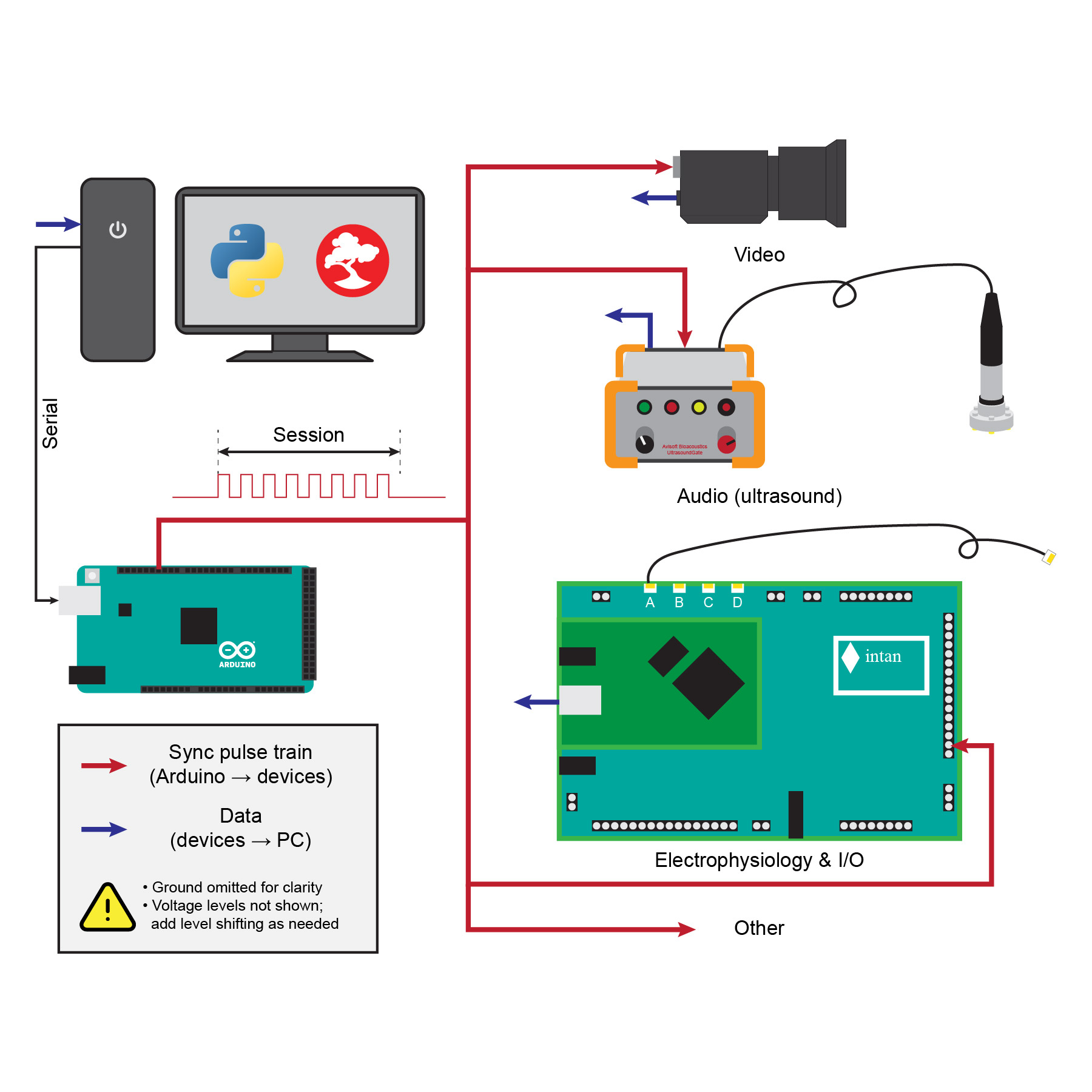
Here, we describe a modular approach for synchronized multimodal data acquisition (Figure 1). Each recording session is organized around a shared external digital sync pulse train. Rather than treating any individual device clock as the reference, a dedicated pulse generator sends the same periodic signal to all participating acquisition systems. Each device either uses this signal to trigger acquisition directly or records the signal alongside its own data stream. The shared pulse train therefore provides a common temporal reference for the experiment.
In this framework, a session is defined by the sync pulse train itself. The first valid sync pulse marks session time t = 0. Subsequent pulses define the session timebase by their pulse index. For a sync rate denoted sync_rate, pulse i occurs at session time i / sync_rate. A session with N pulses therefore has a sync-defined duration of N / sync_rate. Data recorded before the start of the first pulse or after the end of the sync pulse train are considered outside the session.
Different modalities capture the sync reference in modality-specific ways. For example, video cameras can be hardware-triggered so that each sync pulse produces one frame. Audio recordings can embed the pulse train as a digital signal in the audio stream. Electrophysiology, photometry, and other analog or digital signals can be recorded through DAQ systems that capture the pulse train on a digital input channel. The same scheme can be extended to any device that can either accept the sync pulse as a trigger or record it as a digital reference signal.
After acquisition, a validation script extracts or counts the sync reference from each data stream and checks that the session is internally consistent. The resulting pulse and frame indices are used to build lookup tables that map modality-specific samples or frames onto the shared session timebase. These mappings allow continuous signals, detected events, and other derived measurements from independently recorded streams to be compared on a common session clock.
The sections below describe the hardware and software components that implement this design. We first describe how the sync pulse train is generated and controlled. We then describe the modality-specific acquisition modules currently used for video, audio, and electrophysiology; the same synchronization logic can be extended to additional devices. We next describe the recording workflow and session data organization. Finally, we describe the post-hoc validation and timing-conversion steps used to map recorded data onto the shared session timebase. As a practical guide, each section includes an approximate setup time in the margin for a smooth setup.
The examples below use devices we currently use in the Banerjee Lab, including FLIR machine-vision cameras, Avisoft UltraSoundGate audio interfaces, and an Intan acquisition board. We describe these systems in detail because they are the setups we have tested most extensively, but the synchronization strategy is not tied to these exact devices. Any camera, audio system, DAQ, or behavioral controller that can record or respond to a shared timing signal can fit into the same general framework. Devices that cannot directly accept or record a digital sync line may still be synchronized through an observable timing marker, such as an LED visible to a camera, although those adaptations are outside the main scope of this protocol.
Figure 1. Schematic overview of the synchronization design
An Arduino-controlled digital pulse train defines the session timebase and is distributed to each acquisition device. Each modality captures this shared temporal reference in a modality-specific form, enabling post-hoc validation and alignment to a common session clock.
Shared Pulse Train Generation and Control (Arduino + Bonsai)
1h
Overview of pulse control
In this section, we set up a Windows PC to control the shared synchronization signal used during acquisition. The PC communicates with an Arduino microcontroller over a serial connection, and the Arduino generates the digital pulse train that defines the experimental session timebase. We first test pulse control directly from the Arduino IDE using an LED and an intentionally slow blink pattern, then reproduce the same start/stop control from a simple Bonsai workflow. This provides a minimal working example of serially controlled pulse generation before the same Bonsai control logic is incorporated into the full acquisition workflow.
Basic software setup
Before setting up the acquisition workflow, install and configure a few basic development tools on the Windows acquisition computer:
- Visual Studio Code for editing code and configuration files
- Git for working with the repository
- Miniconda for creating the Python environment used by the acquisition scripts
Additional device-specific software will be installed in the sections where each modality is configured.
For this protocol, users should be comfortable with basic command-line navigation and commands as they go, whether in Bash, Windows PowerShell, or a similar shell. For conda-specific commands, the official conda cheatsheet is a useful quick reference.
10m
Clone the repository
This protocol is accompanied by a companion code repository. The repository has two related but separable parts: acquisition/ for Arduino, Bonsai, and Python acquisition assets, and sync_analysis/ for session validation, sync extraction, timebase mapping, and demo analysis. The codebase is a fresh, protocol-oriented implementation of workflows used in the Banerjee lab, intended to make the synchronization logic easier to install, read, and adapt. Please contact us by email or open a GitHub issue if questions or problems come up.
Open the Anaconda PowerShell Prompt from the Windows Start menu: Start → Miniconda3 (64-bit) → Anaconda PowerShell Prompt (miniconda3). For convenience, this shortcut can be copied to the desktop.
In the prompt, navigate to the folder where the repository will be stored. For example:
If prompted to log in to GitHub, follow the instructions shown in the terminal.
5m
Prepare Arduino
Prepare an Arduino Mega 2560 Rev3, or another Arduino-compatible board with USB serial communication and digital output pins, and a basic electronics starter kit. Download and install the Arduino IDE. We will use it to upload the sync pulse generator firmware to the Arduino and to test serial control before moving to Bonsai.
5m
Build the Arduino sync test circuit
Connect an LED circuit to the Arduino so the sync output can be inspected visually. Here we use digital pin 11 as the sync output pin. Connect pin 11 to a current-limiting resistor, then connect the resistor to the long leg of the LED. Connect the short leg of the LED to Arduino GND (Figure 2). In later steps, we will build on top of this same circuit to distribute the sync signal to acquisition devices, while keeping the LED as a simple visual indicator of whether the pulse train is running. The sync pulse can also be inspected directly by connecting the output signal and ground to an oscilloscope.
Figure 2. Arduino LED test circuit
Digital pin 11 is connected through a current-limiting resistor to an LED, with the LED returning to Arduino GND.
Open the sync pulse generator sketch in the Arduino IDE:
acquisition/arduino/sync_pulse_generator/sync_pulse_generator.ino
The sketch uses simple serial commands to control the pulse train. Sending 1 enables the pulse train. Sending 0 stops the pulse train and holds the sync output low. The output pin is set by syncPin, and the pulse timing is set by pulseHighUs and pulseLowUs.
For the first visual test, temporarily slow down the loop by replacing the two delayMicroseconds(...) lines with delay(1000). This makes the LED blink slowly enough to see clearly.
Connect the Arduino to the computer with a USB cable. In the Arduino IDE, select the board type under Tools -> Board, then select the serial port under Tools -> Port. If multiple serial devices are connected, choose the port corresponding to this Arduino and note the port name, such as COM3, because the same port will be used later from Bonsai. Upload the temporary slow-blink version of the sketch to the Arduino.
After uploading, open the Arduino IDE Serial Monitor and set the baud rate to 9600. Send 1 to start the blinking pulse train. The LED should blink on and off once per cycle. Send 0 to stop the pulse train. The LED should turn off (Video 1).

Video 1. Serial control of the Arduino sync output
Sending 1 in the Arduino IDE Serial Monitor starts a slow LED blink, and sending 0 stops the output.
After confirming serial control with the slow blink test, restore the original delayMicroseconds(pulseHighUs) and delayMicroseconds(pulseLowUs) lines and upload the sketch again. At the default 50 Hz sync rate, the LED will appear continuously on while the pulse train is running and off when it is stopped.
This test confirms that the Arduino can generate the sync output and that the pulse train can be controlled over serial. In the next step, we will reproduce the same serial start/stop control from Bonsai.
20m
Control the pulse train from Bonsai
Bonsai is a visual reactive programming environment commonly used in neuroscience for coordinating hardware control, data acquisition, and real-time data processing. Here, we use Bonsai as a simple orchestration layer for the Arduino sync pulse generator. The goal is to reproduce the same serial start/stop control tested in the Arduino IDE, then build on this workflow in the next section to coordinate video acquisition from the FLIR camera.
Download and install Bonsai on the Windows acquisition computer. After installation, open Bonsai from the Start menu, and optionally copy the Bonsai shortcut to the desktop for convenience. In Bonsai, open Manage Packages and install the Bonsai Starter Pack, which includes the packages needed for this simple keyboard-input and serial-control workflow.
Open the Bonsai pulse-control workflow:
acquisition/bonsai/workflows/simple_pulse_control.bonsai
Figure 3. Bonsai workflow for serial pulse control
Keyboard events send serial commands to the Arduino: T sends 1 to start the pulse train, and F sends 0 to stop it.
This workflow maps two keyboard events to serial commands (Figure 3). Pressing T sends 1 to the Arduino and starts the pulse train. Pressing F sends 0 to the Arduino and stops the pulse train. Each control branch uses a KeyDown node to detect the key press, a string value (1 or 0) as the command, and a SerialWriteLine node to send the command to the Arduino over the selected COM port. Before running the workflow, confirm that the PortName in both SerialWriteLine nodes matches the Arduino port used in the Arduino IDE, such as COM3. Close the Arduino IDE Serial Monitor so Bonsai can access the serial port.
Run the Bonsai workflow by clicking Start. Click inside the Bonsai workflow window so it has keyboard focus, then press T to start the Arduino pulse train. The LED should appear on while the pulse train is running. Press F to stop the pulse train; the LED should turn off. When the pulse train is off, click Stop to stop the Bonsai workflow (Video 2). This confirms that Bonsai can control the Arduino over serial, using the same start/stop logic that will be incorporated into the full acquisition workflow.

Video 2. Bonsai control of the Arduino sync output
Pressing T in Bonsai sends 1 to the Arduino and starts the 50 Hz sync pulse train; pressing F sends 0 and stops the output.
20m
Video Acquisition (FLIR)
1h
Overview of video acquisition
Video is a sequence of image frames acquired at specific times. To align video with other data streams, such as audio, electrophysiology, or behavioral events, we need to know how each video frame maps onto the shared session timebase. This can be done either by using an external signal to trigger frame acquisition, or by recording a timing signal that indicates when each frame is captured. The camera therefore needs to support timing input or output through hardware trigger lines.
In this protocol, we use a FLIR Blackfly S machine vision camera and trigger frame acquisition with the shared Arduino sync pulse train. Each rising edge of the sync pulse triggers one camera frame. With a 50 Hz sync train, the camera acquires one frame per pulse, producing a 50 fps video whose frame index is tied directly to the session pulse index. Because raw video data become large quickly, we also encode the video during acquisition rather than saving raw frames.
We first configure the camera in SpinView, the graphical camera-control application included with the Spinnaker SDK, to set basic acquisition parameters and enable external triggering. We then use Bonsai to coordinate Arduino pulse control and camera acquisition in a single workflow. Finally, we use a Python wrapper to launch the Bonsai workflow and pipe raw frames into ffmpeg, allowing video to be encoded on the fly with flexible parameters. The example below uses one FLIR Blackfly S camera, but the same approach can be extended to multiple synchronized cameras.
Set up the camera
Select a camera and lens based on the imaging needs of the behavioral setup. For the camera, important parameters include resolution, maximum frame rate at the selected resolution, monochrome versus color imaging, shutter type, interface bandwidth, trigger I/O support, and lens mount. For the lens, consider field of view, working distance, aperture, depth of field, and distortion. Monochrome cameras are usually the simpler choice for infrared illumination; color cameras may require additional consideration because of Bayer sampling and IR-cut filtering. In this protocol, we demonstrate the workflow with a FLIR Blackfly S monochrome USB3 camera (BFS-U3-20S4M-C) and a 4.5 mm C-mount lens (Edmund Optics #86-900), but other machine vision cameras and lenses with hardware trigger support can be used.
Mount the camera and lens in the recording setup, and attach the GPIO cable to the camera. Leave the USB cable disconnected for now; we will connect the camera to the acquisition computer after installing Spinnaker/SpinView in the next step. Lens focus and aperture will be adjusted later using the live camera view in SpinView.
The GPIO cable carries the hardware trigger signal into the camera. For the FLIR Blackfly S camera and GPIO cable used here, we follow the Teledyne synchronized-capture wiring guide. The guide describes the GPIO pinout and wiring logic for several FLIR camera families. In our setup, the Arduino sync pulse acts as the external trigger source, so the Blackfly S camera is wired like a secondary camera receiving a trigger signal. Connect the Arduino sync output to the camera trigger input wire, and connect Arduino GND to the camera ground wire. With the Blackfly S camera and GPIO cable used here, this means connecting Arduino sync output pin 11 to the green wire and Arduino GND to the brown wire (Figure 4). Confirm the pin and wire-color mapping for the exact camera and GPIO cable being used before relying on this wiring for acquisition.
Figure 4. FLIR camera trigger wiring
The Arduino sync output is routed through the breadboard to the FLIR Blackfly S GPIO trigger input, with shared ground connected between the Arduino and camera. The LED remains in the circuit as a visual indicator of the sync pulse train.
15m
Configure the camera in SpinView
Install the Teledyne FLIR Spinnaker SDK on the Windows acquisition computer. The SDK includes SpinView, the graphical application we will use to configure and test the camera. Downloading Spinnaker may require creating or signing into a Teledyne account. For this protocol, install the Windows 64-bit Spinnaker SDK 1.29.0.5, which is compatible with Bonsai.Spinnaker 0.7.1. During installation, choose Application Development as the installation type so the SDK components needed by Bonsai are installed.
Note
Spinnaker Version Compatibility
Bonsai.Spinnaker must be used with a compatible Spinnaker SDK version. Although newer Bonsai.Spinnaker releases support the Spinnaker 4.x series, the specific older 4.x SDK release required by Bonsai may not always be available from Teledyne’s download page. To keep the protocol reproducible, we use the older compatible pair: Spinnaker SDK 1.29.0.5 and Bonsai.Spinnaker 0.7.1.
After installing Spinnaker/SpinView, connect the camera to the acquisition computer with the USB3 cable and open SpinView. The camera should appear in the device list. Start streaming with trigger mode off so the camera free-runs. Use this live view to position the camera, adjust the lens focus and aperture, and tune the image acquisition settings (Figure 5).
In the Settings tab, use fixed manual settings for acquisition. In a stable recording setup, lighting and camera placement are usually held constant within a session and across related sessions, so automatic camera adjustments can introduce unwanted variability. Disable automatic exposure and gain, then adjust Exposure Time and Gain for the actual recording conditions. If using a color camera, also set white balance manually. Gamma can also be enabled or disabled and tuned here, but once chosen it should be kept fixed for the experiment. Check the Device Link Throughput Limit and make sure it is high enough that USB bandwidth will not limit acquisition.
In the Image Format tab, confirm the image size and pixel format. The default image size is usually appropriate, but the pixel format should be checked because it determines how frames will be interpreted later by Bonsai, Python, and ffmpeg. For the monochrome Blackfly S camera used here, Mono8 is a good default.
Once the live image looks good, stop streaming and configure the trigger settings in the GPIO tab, following the FLIR synchronized-capture guide for a secondary camera. For the Blackfly S camera used here, set Trigger Source to Line 3, set Trigger Overlap to Read Out, and set Trigger Mode to On. The trigger will use the rising edge of the sync pulse to start frame acquisition.
Figure 5. SpinView camera configuration interface
SpinView is used to preview the camera stream, set acquisition and image-format parameters, configure GPIO triggering, and save the camera settings profile.
Test the trigger configuration before saving it. Start streaming in SpinView while the Arduino pulse train is off. No image should appear because the camera is waiting for external triggers. Start the Arduino sync pulse train using the previous serial or Bonsai control workflow. The SpinView image should update at the sync rate. Stop the pulse train, and the image should freeze.
When the settings are correct, use Save Camera Settings Profile in SpinView to save the configuration. This saves the acquisition, image format, and trigger settings so the configuration can be reloaded for later acquisition. It is also recommended to write down the edited camera settings, so the configuration can be reproduced later if the saved camera profile is lost or overwritten.
15m
Monitor triggered video in Bonsai
Next, we extend the Bonsai pulse-control workflow so Bonsai can also acquire and display triggered camera frames. This step confirms that Bonsai can coordinate the Arduino sync pulse train and the FLIR camera in one workflow before we add video writing.
In Bonsai, open Manage Packages and install Bonsai.Spinnaker. For this protocol, install Bonsai.Spinnaker 0.7.1, which is compatible with Spinnaker SDK 1.29.0.5. This version pairing should match the Spinnaker/SpinView installation used to configure the camera.
Open the triggered video monitoring workflow:
acquisition/bonsai/workflows/triggered_video_monitor_v1.bonsai
Figure 6. Bonsai workflow for triggered video monitoring
The workflow combines Arduino serial pulse control with FLIR camera monitoring. The upper branches send 1 or 0 to the Arduino to start or stop the sync pulse train, while the SpinnakerCapture node displays camera frames triggered by the sync pulses.
This workflow (Figure 6) builds on the previous serial pulse-control workflow. The T key still sends 1 to the Arduino to start the sync pulse train, and the F key still sends 0 to stop it. The new part is a SpinnakerCapture node connected to an Image output, allowing Bonsai to display frames from the FLIR camera as they are triggered.
Before running the workflow, confirm that the Arduino serial port in both SerialWriteLine nodes matches the port used earlier, for example COM3. In the SpinnakerCapture node, set SerialNumber to match the camera shown in SpinView, and set ColorProcessing to NoColorProcessing. Start the Bonsai workflow by clicking Start. Double-click the Image node to open the image visualizer. With the sync pulse train off, no image should appear because the camera is waiting for external frame triggers. Press T to start the Arduino pulse train; the live video should update in the image visualizer. Press F to stop the pulse train; the video should freeze. Once the pulse train is stopped, click Stop to stop the Bonsai workflow.
This confirms that Bonsai can coordinate serial control of the Arduino and triggered image acquisition from the FLIR camera. In the next step, we will use a related Bonsai workflow with a Python wrapper to pipe the triggered frames into ffmpeg for video writing.
10m
Run triggered video acquisition with Python and ffmpeg
So far, Bonsai can control the Arduino sync pulse train and display camera frames triggered by that pulse train. The next step is to write those frames to disk in a reproducible way. Saving raw frames directly would produce very large files, so we use ffmpeg to encode the video during acquisition. To keep the workflow flexible across rigs and recording formats, we use a Python wrapper script to connect the acquisition config, Bonsai workflow, and ffmpeg encoding process. This design is adapted from Point_Grey_Bonsai_multi_camera_acquisition by Thomas Akam, with changes for the sync-triggered acquisition scheme used here.
20m
Create the acquisition environment
First, create the acquisition conda environment. Open the Anaconda PowerShell Prompt, navigate to the repository folder, and run:
conda env create --prefix $HOME/.conda/envs/multimodal-sync-acquisition -f acquisition/envs/acquisition.yaml
conda activate $HOME/.conda/envs/multimodal-sync-acquisition
This environment provides Python for running the acquisition wrapper script and ffmpeg for video encoding installed from conda-forge. Camera control still depends on the external Windows software configured above, including Spinnaker/SpinView, Bonsai, and Bonsai.Spinnaker. For rigs that require older ffmpeg/NVENC behavior, the repository also includes a legacy ffmpeg 4.2.2 environment:
acquisition/envs/acquisition_legacy_ffmpeg422.yaml
Note
NVIDIA/FFmpeg compatibility
This protocol uses GPU video encoding through FFmpeg’s h264_nvenc encoder. The working combination depends on the FFmpeg build, NVIDIA driver, GPU model, and encoder options, so each acquisition computer should be tested with a short representative recording before long sessions. In our tests, a GeForce RTX 3060 with NVIDIA driver 581.57 worked with conda-forge FFmpeg 8.1.1 and the modern config. A Quadro RTX 4000 with NVIDIA driver 516.94 worked with FFmpeg 4.2.2 and the legacy config. These examples are starting points; if encoding fails, playback is incompatible, file size changes unexpectedly, or GPU load is too high, adjust the FFmpeg version, NVIDIA driver, or video.ffmpeg_output_options in the acquisition config.
Review the config, Bonsai workflow, and Python wrapper
The acquisition step is controlled by three linked pieces: a YAML config, a Bonsai workflow, and a Python wrapper script. The config records the rig-specific settings, the Bonsai workflow handles camera acquisition and the named-pipe output, and the Python script connects Bonsai to ffmpeg for video encoding. Keeping these pieces separate makes the workflow easier to reuse: the same script can run different rigs by changing the config, while the Bonsai workflow remains responsible for hardware-facing acquisition.
The example config is:
acquisition/configs/example_v1_50hz.yaml
This file describes the one-camera, 50 Hz video acquisition example. The session.sync_rate_hz field records the sync pulse rate and is used as the video frame rate for ffmpeg encoding. The paths section points to the output data folder, the Bonsai executable, and the Bonsai workflow to launch. The video section specifies the frame size, raw input pixel format, output-side ffmpeg options, pipe wait timeout, segmentation settings, and camera list. The video.ffmpeg_output_options block is passed directly to ffmpeg, which lets different rigs use different encoder settings without changing the Python wrapper.
The Bonsai workflow used by this config is:
acquisition/bonsai/workflows/triggered_video_writer_v1.bonsai
Figure 7. Bonsai workflow for triggered video writing
The workflow sends serial start/stop commands to the Arduino and acquires frames from one FLIR camera. The camera branch writes triggered raw frames to a Windows named pipe, which the Python wrapper connects to ffmpeg for video encoding.
This workflow (Figure 7) extends the triggered video monitoring workflow from the previous step. It still uses the T and F keys to send serial start/stop commands to the Arduino, but instead of only displaying frames, it writes raw camera frames to a Windows named pipe. The camera acquisition branch is packaged as Box1, which contains one SpinnakerCapture node. When the workflow is launched by Python, the camera serial number from the config is passed into Box1. Frames from Box1 are then sent to an ImageWriter node that writes to \\.\pipe\videopipe1. The _v1 suffix indicates that this workflow is wired for one video stream.
The Python wrapper script is:
acquisition/scripts/run_acquisition.py
This script is the main entry point for running the acquisition from the command line. It reads the YAML config, prints the acquisition settings, launches the Bonsai workflow, waits for the named pipe to appear, and then starts ffmpeg. ffmpeg reads raw frames from the pipe and encodes them directly to video during acquisition. With the default config, the output video filename has the form:
<camera_name>_<timestamp>.mp4
Run the acquisition wrapper
Run the acquisition wrapper from the repository root with the acquisition conda environment active:
python acquisition/scripts/run_acquisition.py -c acquisition/configs/example_v1_50hz.yaml
The script will print the config path, output folder, Bonsai workflow, effective video settings, camera serial number, named pipe, Bonsai command, and ffmpeg command. Check this output before starting the recording. In particular, confirm that the camera serial number matches SpinView, the Bonsai executable path is correct, the output folder is correct, and the named pipe is \\.\pipe\videopipe1.
After the script launches Bonsai, the Bonsai workflow window should open. Double-click the Image node in the Bonsai workflow to open the image visualizer. At this point, the sync pulse train should still be off, so no image should appear and the sync indicator LED should be off. The Python terminal should report that ffmpeg has started for cam0 once Bonsai opens the video pipe. Press T in the Bonsai workflow to start the Arduino pulse train and begin sending triggered frames through the pipe. The sync indicator LED should turn on, and the live video should update in the image visualizer.
To stop the recording, press F in the Bonsai workflow to stop the Arduino pulse train. The live video should freeze, and the sync indicator LED should turn off. Once the pulse train is stopped, click Stop in Bonsai to stop the workflow, then close the Bonsai window. The Python script will return to the command prompt, and the encoded video should be finalized in the configured output folder with a filename of the form: cam0_<timestamp>.mp4 (Video 3).

Video 3. Python-controlled triggered video acquisition
The Python wrapper launches the Bonsai workflow, waits for the video pipe, and starts ffmpeg encoding. Press T in Bonsai to start the Arduino sync pulse train and triggered video acquisition. Press F to stop the pulse train, then stop and close the Bonsai workflow.
Note
GPU video encoding settings
This workflow uses FFmpeg with the NVIDIA h264_nvenc encoder to compress video during acquisition. The modern example config keeps the encoder settings simple, using preset: p4 and pix_fmt: yuv420p for speed and playback compatibility. More FFmpeg options can be added under video.ffmpeg_output_options if a rig needs different quality, file size, or throughput behavior. For multi-camera rigs, monitor GPU video encode usage during a short test recording before running long sessions.
Note
Sync-rate calibration
The Arduino pulse timing constants in the sync-pulse sketch were empirically tuned against Bonsai timestamp logs from the triggered-video workflow. If you change the Arduino board, firmware timing, or sync rate, verify the realized pulse/frame rate with a short test recording and update the firmware and config values accordingly.
Optional acquisition variants
The one-camera monochrome example is the simplest version of the acquisition pipeline. The same structure can be adjusted for long recordings, color cameras, or multiple synchronized cameras by changing the acquisition config and, when needed, the Bonsai workflow.
Note
Long recordings
To split a long recording into multiple video files, use ffmpeg segmentation through the acquisition config. Set segment_seconds in the YAML file to the desired segment length in seconds. For example, segment_seconds: 3600 writes one-hour video files. See: acquisition/configs/example_v1_50hz_1h_segments.yaml. The output filenames will have the form:
<camera_name>_<timestamp>_%05d.mp4.
Note
Color cameras
For color machine-vision cameras, the raw frames are often Bayer encoded rather than RGB. In SpinView, confirm the camera pixel format, for example BayerRG8. In Bonsai, keep the raw Bayer image stream connected to the named-pipe ImageWriter, so ffmpeg receives the original raw frame data. For visual monitoring, add a separate branch from the image stream through a ConvertColor node, using a conversion such as BayerRG2RgbVng, and connect that converted output to an Image visualizer. In the acquisition config, set input_pixel_format to the matching ffmpeg pixel format, for example bayer_rggb8.
Note
Multiple cameras
For multiple cameras, use a Bonsai workflow with one camera branch per video stream. Starting from the one-camera writer workflow, add additional camera boxes such as Box2, Box3, and so on. Each box should contain its own SpinnakerCapture branch and write to a distinct named pipe, for example \\.\pipe\videopipe2 and \\.\pipe\videopipe3. In the acquisition config, add one camera entry per camera in the same order as the Bonsai boxes: the first camera entry maps to Box1, the second maps to Box2, and so on. For each camera, set the correct name, serial_number, pipe_name, and enabled fields. The pipe_name in the config must match the ImageWriter pipe path in the corresponding Bonsai branch. For multi-camera rigs, also make sure the computer has enough USB bandwidth; if the built-in ports are not sufficient, a PCIe USB host controller card, such as the Teledyne USB 3.1 host controller card, can be added to provide additional USB controllers for the cameras.
For a concrete two-camera color example with one-hour video segments, see acquisition/configs/example_v2_50hz_1h_segments_legacy_ffmpeg422.yaml and acquisition/bonsai/workflows/triggered_video_writer_v2.bonsai.
Audio Acquisition (Avisoft Bioacoustics)
50m
Overview of audio acquisition
Behavioral experiments often use audio recording to capture vocalizations and other sound-producing events. Sound is a pressure signal that changes over time, and digital audio represents this signal by sampling the waveform at a fixed sampling rate. For rodent vocalization experiments, these recordings often need to capture ultrasonic frequencies, so the microphone and recording interface must support higher bandwidth and higher sampling rates than typical human-audio equipment.
In this protocol, we use an Avisoft Bioacoustics UltraSoundGate system for ultrasonic audio recording. These systems are commonly used in bioacoustic studies because they support high-sample-rate recording and are designed for sensitive ultrasonic microphones with broad frequency response. As with video, the audio recording is acquired by its own hardware and software, so it needs a way to be aligned with the shared session timebase.
Avisoft describes several approaches for synchronizing UltraSoundGate recordings with video or physiology recordings in its UltraSoundGate synchronization guide. Here, we use the UltraSoundGate digital input to record the Arduino sync pulse train directly into the audio file. RECORDER USGH stores this digital input state in the least significant bit of the 16-bit audio samples. After acquisition, the audio waveform and embedded LSB sync track can be extracted from the same WAV file, allowing audio samples to be mapped onto the shared session clock.
Set up the Avisoft audio hardware
In this protocol, we record ultrasonic audio with an Avisoft UltraSoundGate 116H and an Avisoft CM16/CMPA condenser ultrasound microphone. The UltraSoundGate 116H is a single-channel USB recording interface for high-sample-rate ultrasound acquisition, and the CM16/CMPA microphone is designed for ultrasonic recording with broad frequency response and high sensitivity. The 116H also has a TTL-compatible digital input, which we will use to record the Arduino sync pulse train alongside the audio.
Connect the CM16/CMPA microphone to the UltraSoundGate 116H using the XLR microphone cable. Mount the microphone in the recording rig so it has a clear acoustic path to the animal or sound source; the microphone is directional, so placement and orientation affect the recorded signal. Place the UltraSoundGate 116H near the sync circuit and somewhere accessible for later gain adjustment. Leave the USB cable disconnected for now; we will connect the 116H to the acquisition computer after installing and configuring the Avisoft recording software. Gain will be adjusted later using the live level display in RECORDER USGH.
To route the sync signal into the 116H, connect the Arduino sync output circuit to the 116H digital input using a 2.5 mm mono plug cable, such as Tensility 10-00343 (Figure 8). Use the 116H digital input/DIN connector for this step, not the TRG or SYNC connector. The digital input carries the same sync pulse train used to trigger the camera, allowing RECORDER USGH to store the pulse state in the audio file. For a 2.5 mm mono plug, the tip is normally the signal contact and the sleeve is normally ground; use a multimeter to confirm which cable lead connects to each contact before wiring. Connect the tip/signal lead to the Arduino sync output, and connect the sleeve/ground lead to Arduino GND. Make sure the Arduino and UltraSoundGate digital input share a common ground. This completes the hardware path needed for embedding the sync pulse train in the audio recording.
Figure 8. Avisoft audio hardware and sync input wiring
The CM16/CMPA microphone is connected to the UltraSoundGate 116H, and the Arduino sync output is routed to the 116H digital input through a 2.5 mm mono plug cable.
15m
Configure RECORDER USGH
Install Avisoft RECORDER USGH on the Windows acquisition computer from the Avisoft downloads page. We also recommend installing Avisoft SASLab Lite, which is useful for quickly opening and inspecting recorded WAV files. Avisoft provides detailed documentation for RECORDER in the Avisoft-RECORDER manual; here, we only highlight the settings that matter for embedding the sync pulse train in the audio recording. After installation, connect the UltraSoundGate 116H to the computer with USB and open RECORDER USGH (Figure 9).
Open the configuration window from Options -> Configuration. In Channel Settings, choose the base directory where WAV files will be saved. If recording from multiple microphone channels, set clear channel names so the output files can be identified unambiguously. In the Trigger settings, set the trigger mode to permanent (unlimited) and set both pre-trigger and post-trigger durations to 0. In this protocol, RECORDER USGH should write continuously while the sync pulse train defines the true session start and stop.
In Input Device Settings, confirm that the selected device is the UltraSoundGate 116H. Set the sampling rate and recording format for the experiment. For the example workflow used here, set the sampling rate to 250 kHz. If a different sampling rate is used, update the downstream analysis config accordingly. For sync extraction from the digital input, use a 16-bit WAV format so the least significant bit can store the DIN state. Open the device Settings dialog and enable Keep DIN, Show DIN, and Ignore GetOverlappedResult error.
Next, configure file naming and file length. In Filenames, enable date-based filenames and compact date formatting. This produces filenames that are easy to sort and match the downstream session validation workflow used here. For long recordings, set Maximum file size by recording length. WAV files have a maximum size limit, so splitting long sessions into multiple files avoids oversized recordings. A 60-minute maximum length is a practical default because it keeps individual WAV files manageable while preserving continuous recording across the session.
When the settings are complete, save the RECORDER USGH configuration using Save or Save As. Saving the configuration helps keep the directory, trigger mode, sample rate, and DIN settings reproducible.
Figure 9. RECORDER USGH configuration for audio sync recording
RECORDER USGH is configured for continuous 16-bit audio recording from the UltraSoundGate 116H, with the digital input retained and displayed so the Arduino sync pulse train is embedded in the WAV file.
After saving the configuration, use the live level display in RECORDER USGH to adjust the microphone gain for the recording setup. Set the gain under the expected recording geometry and sound conditions, and avoid settings that clip loud sounds. Once chosen, keep the gain fixed across comparable sessions.
15m
Record audio with the embedded sync pulse
For audio acquisition, start the audio recording before starting the sync pulse train, and stop the audio recording after stopping the sync pulse train. This order intentionally sandwiches the sync-defined session inside the WAV file. The audio file therefore contains a short pre-session period, the full sync pulse train, and a short post-session period. This makes the first and last sync pulses easy to detect during validation and avoids losing the beginning or end of the session because of small delays in manually starting or stopping software.
In RECORDER USGH, start file writing first. Confirm that the software is actively recording to the intended output directory. Then start the Arduino sync pulse train from the Python-launched Bonsai workflow, the simpler Bonsai pulse-control workflow, or the Arduino IDE Serial Monitor. After the sync pulse train starts, the sync indicator LED should turn on, and the blue DIN indicator in RECORDER USGH should alternate on and off with the pulse train. During the session, RECORDER USGH records the microphone signal while also embedding the digital input state in the least significant bit of the audio samples. At the end of the session, stop the Arduino sync pulse train first. After the sync indicator LED turns off, stop recording in RECORDER USGH.
The order is therefore:
Start audio recording -> start sync pulse train -> stop sync pulse train -> stop audio recording
This workflow ensures that the sync pulse train is fully contained within the audio file. In downstream validation, the recorded LSB pulse train can then define the audio session boundary and map audio sample indices onto the shared session timebase.
10m
Visualize the embedded audio LSB sync track
This example visualization helps show how the audio sync signal is stored in the recorded WAV file. Run this notebook from the sync_analysis environment with the all dependencies installed. In an example audio file recorded this way, the embedded sync track can be inspected with the notebook:
sync_analysis/notebooks/inspect_audio_lsb_sync.ipynb
The notebook loads the WAV file as 16-bit integer samples, extracts the least significant bit from the selected audio channel, and plots the acoustic waveform together with the extracted LSB sync track. The full-recording view shows where the sync pulse train begins and ends within the audio file, and the zoomed view around the first transition shows the square-wave pulse train directly (Figure 10). From this extracted LSB track, we can detect the rising edges of the sync pulses, which will be used in later sections for session validation and mapping audio samples onto the shared session timebase.
Figure 10. Embedded audio LSB sync track
The Avisoft WAV file contains both the acoustic waveform and the embedded digital sync signal. The extracted least significant bit shows the Arduino sync pulse train recorded through the UltraSoundGate digital input.
10m
Electrophysiology and I/O Acquisition (Intan Technologies)
45m
Overview of electrophysiology and I/O acquisition
Electrophysiology and other DAQ-based recordings often include continuous neural signals together with auxiliary input channels for behavioral events, stimulation timing, or other external signals. For synchronization, the key requirement is that the DAQ system records the shared sync pulse train in the same timebase as the neural or analog signals. A dedicated digital input channel is well suited for this because each sample of the digital channel records whether the sync line is low or high.
In this protocol, we demonstrate this idea with an Intan RHD USB interface board for electrophysiology and general I/O recording. This board has been discontinued, but it remains a useful example of a DAQ system that records amplifier data and digital inputs together. The same synchronization logic can be applied to other acquisition systems, such as the Open Ephys Acquisition Board with I/O hardware, or pyPhotometry for fiber photometry, as long as the system can record an external digital input alongside its primary data stream.
Here, we route the Arduino sync pulse train into one DAQ digital input channel. During acquisition, the DAQ records neural or analog signals while also recording the sync pulse state on that digital input. After acquisition, rising edges in the recorded digital input channel can be detected and used to map ephys, photometry, or other DAQ samples onto the shared session timebase.
Set up the DAQ sync input hardware
Before connecting the Arduino sync output to an electrophysiology or DAQ system, check the voltage level expected by the DAQ digital input. The Arduino sync output used here is a 5 V digital signal, while some DAQ inputs expect 3.3 V logic. For this protocol, we step the Arduino sync signal down to approximately 3.3 V before routing it to the DAQ digital input.
Build a simple voltage divider on the breadboard using two resistors with a 1:2 ratio, for example 1.1 kΩ and 2.2 kΩ. Connect the Arduino sync output to the 1.1 kΩ resistor, connect the other end of that resistor to the divider output node, and connect the 2.2 kΩ resistor from that node to ground. Connect the divider output node to the DAQ digital input channel. With this resistor ratio, a 5 V Arduino pulse is reduced to approximately 3.3 V at the divider output.
Connect Arduino GND to the DAQ ground so the two devices share a common voltage reference. This common ground is required for the DAQ input to interpret the sync pulse correctly. The final wiring is therefore: Arduino sync output -> voltage divider -> DAQ digital input, with Arduino GND connected to DAQ GND (Figure 11).
Figure 11. Voltage-divided sync input for DAQ recording
The Arduino sync pulse is reduced from 5 V to approximately 3.3 V with a resistor divider, then routed to a DAQ digital input channel. Arduino GND and DAQ GND are connected to provide a common reference.
15m
Configure Intan RHX for sync input recording
Install the Intan RHX data acquisition software from the Intan downloads page. Intan provides an RHX user guide with detailed instructions for the full software interface. Here, we only highlight the settings needed for this protocol: recording the DAQ signals and the Arduino sync pulse train together in the same Intan timebase. After installation, connect USB and power to the Intan RHD USB interface board, then open RHX.
In RHX, confirm that the board is detected and set the acquisition sampling rate. For the example workflow used here, set the sampling rate to 30.0 kHz. If a different sampling rate is used, update the downstream analysis config accordingly. Configure the save directory and file naming so the output files are easy to identify.
Next, configure the recording file format. For this protocol, use One File Per Signal Type. This format keeps each signal class in its own file, which makes it straightforward to locate and extract the recorded digital input signal during downstream validation. Enable and display the digital input channel that is physically connected to the Arduino sync pulse circuit, and confirm that this channel changes state when the sync pulse train is started and stopped (Figure 12).
When the acquisition and digital input settings are correct, save the RHX settings as an XML configuration file. Saving the configuration helps keep the sampling rate, save path, file format, and digital input settings reproducible across sessions.
Figure 12. Intan RHX configuration for sync input recording
RHX is configured to record Intan data with the digital input channel enabled. The Arduino sync pulse train is recorded on a dedicated digital input channel in the same timebase as the electrophysiology or I/O signals.
10m
Record Intan data with the embedded sync pulse
As with audio recording, start Intan data writing before starting the sync pulse train, and stop Intan data writing after stopping the sync pulse train. This sandwiches the sync-defined session inside the recorded Intan files, so the full pulse train is captured on the digital input channel with a short margin before and after the session.
In RHX, start data recording first and confirm that files are being written to the intended output directory. Then start the Arduino sync pulse train from the Python-launched Bonsai workflow, the simpler Bonsai pulse-control workflow, or the Arduino IDE Serial Monitor. During the session, RHX records the electrophysiology and I/O signals while also recording the sync pulse state on the selected digital input channel. At the end of the session, stop the Arduino sync pulse train first. After the sync indicator LED turns off, stop recording in RHX.
The order is therefore:
Start Intan recording -> start sync pulse train -> stop sync pulse train -> stop Intan recording
This ensures that the full sync pulse train is contained within the Intan recording and can later be used to define the session boundary and map Intan samples onto the shared session timebase.
10m
Visualize the recorded Intan digital sync channel
This example visualization helps show how the sync pulse train is stored in the Intan digital input recording. Intan describes the One File Per Signal Type format in its RHD2000 data file formats application note. In this format, board digital input samples are written to digitalin.dat as uint16 values. Each 16-bit word stores the state of digital inputs 0-15 bit-by-bit, and an individual channel can be extracted with a bit mask.
In an example Intan recording collected this way, the digital sync channel can be inspected with the notebook:
sync_analysis/notebooks/inspect_intan_digital_sync.ipynb
The notebook loads digitalin.dat, extracts the selected digital input channel, and plots the digital state over time. The full-recording view shows where the sync pulse train begins and ends within the Intan recording, and the zoomed view around the first rising edge shows the square-wave pulse train directly (Figure 13). From this extracted digital channel, we can detect the rising edges of the sync pulses, which will be used in later sections for session validation and mapping Intan samples onto the shared session timebase.
Figure 13. Recorded Intan digital sync channel
The Intan digitalin.dat file contains the state of the board digital input channels. Extracting the bit corresponding to the sync input reveals the Arduino sync pulse train recorded in the same timebase as the electrophysiology and I/O data.
10m
Recording Workflow and Session Data Organization
Recording workflow
Before starting a session, open the acquisition software for each modality and confirm that the saved configurations are loaded. For a video, audio, and Intan example session, this means checking the FLIR camera settings in Bonsai/SpinView as needed, confirming the RECORDER USGH configuration and output directory, and confirming the Intan RHX configuration, sampling rate, enabled digital input, and output directory. Open an Anaconda PowerShell Prompt, activate the acquisition environment, and navigate to the repository directory.
Start file writing in the independently recording systems first. For this example, start audio recording in RECORDER USGH and start data recording in Intan RHX before starting the sync pulse train. Then run the Python acquisition wrapper for video:
python acquisition/scripts/run_acquisition.py -c acquisition/configs/example_v1_50hz_1h_segments.yaml
When Bonsai opens, double-click the image node if live monitoring is needed. Make sure the Bonsai window is active so it receives keyboard input. Press T in Bonsai to start the Arduino sync pulse train and begin the sync-defined session. At the end of the session, press F in Bonsai to stop the sync pulse train. After the pulse train has stopped, click Stop in Bonsai, close the Bonsai window, and then stop audio and Intan recording. This order keeps the full sync pulse train contained within each independently recorded data stream.
Session data organization
Each recording session should be organized as a self-contained folder containing the raw source data, notes, configuration files, logs, sync outputs, and processed results. This makes the session portable and keeps the acquisition record separate from later analysis. Files written directly by acquisition software should go into raw_<modality> folders and should be treated as read-only after acquisition.
For this protocol, raw data are organized by modality and then by channel or stream ID. For example, audio files are stored under raw_audio/<channel_id>/, video files under raw_video/<camera_id>/, and Intan files under raw_intan/<recording_id>/. A minimal session folder may look like this:
example_session_01/
├── notes.txt
├── logs/
├── raw_audio/
│ └── c1_high/
│ └── *.wav
├── raw_video/
│ └── cam0/
│ └── *.mp4
├── raw_intan/
│ └── /
│ ├── digitalin.dat
│ ├── info.rhd
│ ├── settings.xml
│ └── time.dat
├── sync/
├── processed_audio/
├── processed_video/
└── processed_intan/
The notes.txt file can be used to record session-specific notes and analysis commands. Command outputs and diagnostic messages can be saved in logs/. Later, the session validation step will create a sync/ folder containing extracted sync signals, detected pulse indices, validation summaries, and timing lookup tables. YAML config files describing the session organization and validation settings can also be stored at the session level. Derived outputs from modality-specific analyses should go into processed_<modality> folders.
For a concrete example, see example_session_01 in the attached test_sessions.zip, a short demo session containing one Avisoft audio stream, one FLIR video stream, and one Intan digital input stream recorded from the same Arduino sync pulse train. We use this session in the following sections to demonstrate session validation, sync extraction, timebase mapping, and simple synchronized audio-video analysis. The archive also includes example_session_02, a second demo session with two audio streams and two video streams, which provides an additional example of the same validation workflow on a different rig.
Session Validation and Sync Extraction
10m
Overview of session validation
A behavioral session is defined by the shared sync pulse train. The first valid sync pulse marks session time t = 0, and each later pulse defines a session time by its pulse index. For example, with a 50 Hz sync pulse train, pulse i occurs at session time i / 50 seconds. This sync-defined session clock provides the common timebase used to align audio, video, electrophysiology, and other recorded streams.
Session validation has two goals. First, we check that each sync-aware data stream captured the complete session, rather than a partial, missing, or corrupted version of it. For hardware-triggered video, this means counting video frames, because each sync pulse should trigger one frame. For continuous recordings such as audio or Intan digital input, this means extracting the recorded digital sync signal, detecting its rising edges, and counting valid pulses. In a properly synchronized session, these counts should agree across modalities.
Second, validation creates the information needed to map each data stream onto session time. For pulse-recording modalities, such as audio LSB sync or Intan digital input sync, the extracted sync pulses define a lookup table between source sample indices and session times. For triggered video, the frame index maps directly to session time through the sync rate. During validation, the software also records file organization information for each modality, including how segmented files map onto channel-wide source indices. These file-info tables are used later when analysis is run file by file and the results need to be placed back onto the shared session timebase.
Validate the example session
In example_session_01, video was acquired with hardware triggering, so validation counts the number of frames in the video files. The audio stream contains the Arduino sync pulse train embedded in the least significant bit of the WAV samples, so validation extracts the LSB signal and detects rising edges. The Intan stream records the same sync pulse train on a digital input channel, so validation reads digitalin.dat, extracts the selected digital bit, and detects rising edges.
In our recordings, we occasionally observe rare local defects in Avisoft audio files, such as dropped or scrambled samples. For this reason, the audio sync extraction can optionally infer missing pulse indices from unusually long sync intervals. This correction is channel-specific and is used only when enabled in the analysis config.
Create and activate the analysis environment from the sync_analysis/ folder:
cd sync_analysis
conda env create --prefix $HOME/.conda/envs/multimodal-sync-analysis -f envs/analysis.yaml
conda activate $HOME/.conda/envs/multimodal-sync-analysis
pip install -e ".[all]"
Then run session validation from the repository root:
python sync_analysis/scripts/validate_session.py \
-s /path/to/example_session_01 \
-c /path/to/example_a1v1i_50hz.yaml \
--log-file /path/to/example_session_01/logs/validate_session.log
For the demo session, the final count comparison should look like:
audio:c1_high sync_pulses = 1133
intan:0 sync_pulses = 1133
video:cam0 frames = 1133
Session validation passed: all validation counts match.
The script writes validation outputs to the session’s sync/ folder, including count summaries, pulse diagnostics, per-channel file-info tables, and sync lookup tables for pulse-recording modalities. These outputs are used in the next section to map modality-specific samples, frames, and detected events onto the shared session timebase.
The sync output also lets us compare modality-specific timing against the shared session clock. Each device records data using its own nominal sampling rate or frame rate, but independent device clocks can differ slightly and may drift over long recordings. The recorded sync pulses define a source-to-session mapping for each stream, so downstream analysis does not have to rely only on nominal file timing. This is one of the main advantages of using a recorded hardware sync signal rather than aligning streams only by software start times or file metadata.
Note
Interpreting validation problems
Most sessions should pass validation when all streams capture the full sync pulse train. If there is a large count discrepancy, first check for incomplete recordings, incorrect start/stop order, wrong input channels, trigger wiring issues, or a camera that was not receiving every pulse. If only a small number of pulses are rejected or inferred, the issue may reflect local recording defects such as dropped samples, USB throughput limits, disk write delays, or background system load during acquisition. The validation log reports the size and type of the discrepancy, including rejected pulses, inferred missing pulses, and interval irregularities. Whether a session is still usable depends on the experimental question and how much timing uncertainty is acceptable.
10m
Mapping Data to the Session Timebase
20m
Overview of timebase mapping
After session validation, each modality can be analyzed in the way that best fits that data type. Vocalization detection algorithms can operate on audio files, pose estimation algorithms can operate on video files, spike sorting algorithms can operate on electrophysiology recordings, and photometry or analog-signal analyses can operate on their native sampled traces. These modality-specific analyses should not need to know about the other data streams. Keeping this stage modular makes the workflow easier to debug, reuse, and extend.
The synchronization layer is applied after raw data or analysis outputs have been expressed in the source coordinate system of each channel. In this protocol, we distinguish three coordinate systems. file_local coordinates refer to indices or times within one recorded file. source coordinates refer to channel-wide sample or frame indices after all files for one channel are ordered and concatenated. session coordinates refer to the shared sync-defined session clock. The validation step creates the file-info tables needed to move from file_local to source, and the sync lookup tables needed to move from source to session.
Two common kinds of data can be mapped this way. Continuous signals include raw audio waveforms, video-derived ROI intensity traces, pose coordinates, movement speed, analog input signals, electrophysiology-derived continuous signals, and photometry traces. Discrete events include vocalization bouts, spike times, stimulation events, task events, detected behavioral events, and threshold-defined intervals such as LED or buzzer events. In both cases, the core operation is simple: convert each sample, frame, or event boundary into a source index, then map that source index onto session time using the timebase created during validation.
Map example audio and video events
In example_session_01, the Arduino demo circuit drives an LED and a buzzer at the same time. The LED is visible in the video stream, and the buzzer is captured in the audio stream. This gives a simple ground-truth example for checking that audio-derived and video-derived signals align after mapping to session time.
The notebook:
sync_analysis/notebooks/map_buzzer_led_to_session_timebase.ipynb
demonstrates this workflow. First, the notebook analyzes each modality in its own source space. For audio, it loads the WAV file, computes the audio amplitude, and detects buzzer intervals. For video, it reads the video file, extracts the mean intensity from a manually selected LED ROI, and detects LED-on intervals. These detections are first represented in file-local coordinates, then converted into channel-wide source indices using the validation file-info tables.
For a continuous signal recorded in a pulse-based source channel, such as audio, the mapping uses the extracted sync lookup table:
audio_timebase = SyncTimebase.from_sync_data(
audio_sync_data,
source_rate_hz=audio_sample_rate_hz,
source_index_name="sample",
)
audio_session_signal = map_source_signal_to_session_time(
audio_source_signal,
audio_timebase,
)
For hardware-triggered video, the frame index maps directly to session time because each frame corresponds to one sync pulse:
video_timebase = FrameTimebase(sync_rate_hz=sync_rate_hz)
led_session_signal = map_source_signal_to_session_time(
led_source_signal,
video_timebase,
)
Event intervals are mapped in the same way, using their source start and end indices:
buzzer_events_session = map_event_source_indices_to_session_time(
buzzer_events_source,
audio_timebase,
)
led_events_session = map_event_source_indices_to_session_time(
led_events_source,
video_timebase,
)
After mapping, the audio waveform, video ROI intensity trace, buzzer intervals, and LED intervals can be plotted on the same session-time axis (Figure 14). The buzzer and LED events should overlap because they were generated by the same Arduino program.
Figure 14. Audio and video signals and events mapped to session time
The audio waveform, video LED ROI intensity trace, audio-detected buzzer intervals, and video-detected LED-on intervals are mapped from their original source channels onto the shared session timebase. The buzzer and LED events align after mapping.
10m
Make a synchronized demo video
It is often useful to inspect synchronized raw data directly. Short demo videos can help identify patterns, build intuition, check analysis outputs, and generate hypotheses. However, making these videos manually can be cumbersome because each visual frame must be assembled at the correct session time and then encoded into a playable video file.
The demo-video helper in this repository provides a modular way to do this. A demo video is defined by a session-time clip window and a layout config. The renderer creates a fixed canvas and a fixed session-time timeline. Each visual component follows the same pattern: draw the parts that stay constant once, then update the changing content for each requested session time. Components can therefore represent different modalities, such as video frames, audio waveforms, analog traces, digital signals, or event rasters. The rendered frames are encoded with ffmpeg, and an optional audio track is generated separately and combined with the final video.
For example_session_01, we use a demo-video config that renders one video component and one audio waveform component:
sync_analysis/configs/demo_video/example_video_audio_waveform.yaml
Run the demo-video script from the repository root:
python sync_analysis/scripts/make_demo_video.py \
--session /path/to/example_session_01 \
--session-config sync_analysis/configs/example_a1v1i_50hz.yaml \
--demo-video-config sync_analysis/configs/demo_video/example_video_audio_waveform.yaml \
--clip-start-session-s 0 \
--clip-end-session-s 15 \
--output /path/to/example_session_01/demo_videos/demo_video_0_15.mp4
The output video shows the triggered camera stream and the session-mapped audio waveform on the same session-time timeline, with the corresponding raw audio included as the audio track (Video 4).

Video 4. Session-time demo video of synchronized LED and buzzer events
The demo video renders the camera view and audio waveform from example_session_01 on a shared session-time timeline. The visible LED flashes and audible buzzer events occur together because both were driven by the same Arduino signal.
10m
Acknowledgements
We thank Raimund Specht for help setting up and configuring the Avisoft UltraSoundGate recorders and microphones, and Priyanka Gupta for assistance with the FLIR cameras and for feedback on this protocol. We also thank members of the Banerjee Lab for helpful discussions and suggestions. We thank the creators and maintainers of the open-source software used in this project.